First field application of temperature sensor modules for groundwater flow detection near borehole heat exchanger

Abstract

Here, we present the first application of a temperature sensor module (TSM) for deducing groundwater flow velocity and direction at borehole heat exchangers (BHEs). The TSM maps the horizontal temperature distribution around a BHE. As groundwater flow distorts this temperature distribution, flow velocity and direction can be inferred from the measured temperatures. As modular systems, TSMs can be attached to a BHE at any depth. For the studied BHE, the depths of interest are 82 m and at 94 m. We recorded TSM data for 2 weeks before and during the operation of the BHE. After simulating the working fluid temperature, we model the horizontal temperature distributions using the working fluid temperatures at the depths of interest as input. We use the latter simulations for inferring groundwater flow by minimizing the root mean square error between the measured and simulated temperatures. We obtain a groundwater flow of 0.4 m/day in the NW direction and groundwater flow below the detection limit of 0.01 m to 0.02 m/day at 82 m and 94 m depths, respectively. A flow meter measurement in a nearby groundwater well confirms the flow direction at 82 m but gives an order of magnitude higher velocity, which we attribute to the measurement principle. Moreover, long-term monitoring of a BHE equipped with multiple TSMs could provide information on seasonal variations in groundwater flow, changes in the thermal properties of the BHE filling or changes in the thermal resistance between BHE and ground.

Introduction

For heating and cooling, an increasing number of industrial and multifunctional buildings, e.g., hotels, communal buildings, greenhouses or construction halls, and even city quarters, are being equipped with borehole heat exchanger (BHE) fields (e.g., Fütterer et al. 2011; Omer 2008). The efficiency of an individual BHE mainly depends on (i) geophysical subsurface properties (DGGV 2016), e.g., porosity, permeability and heat conductivity, (ii) the BHE design itself and (iii) the backfill material (Luo et al. 2013; Alberti et al. 2017). However, the efficiency of BHE fields, especially their long-term efficiency, is also affected by the distance between neighboring BHEs (Hellström 1983) and by the overall BHE field geometry (Claesson and Eskilson 1988; de Palya et al. 2012). Moreover, the influence of these factors can significantly increase with groundwater flow. Due to its advective heat transport, groundwater flow also influences the efficiency of a single BHE. However, especially for dense BHE fields, the influence of groundwater flow cannot be underestimated (Diao et al. 2004; Hecht-Mendez et al. 2013). Recent research shows that considering groundwater flow for BHE field design and operation can lead to effective long-term behavior, i.e., to sustainable use of the BHE field (Riveraa et al. 2015).

In other words, the sustainable operation of BHE fields requires knowledge of subsurface groundwater flow. There are different methods for measuring groundwater flow in boreholes; see Morgenstern (2005) or Guaraglia and Pousa (2014) for an overview of these methods. All are based on different physical principles but require open boreholes, which might not be available close to the BHE field of interest. Moreover, characterizing heterogeneous groundwater flow, i.e., heterogeneous aquifers, would require many additional boreholes. Therefore, we developed the temperature sensor module (TSM) for deducing groundwater flow velocity and direction by utilizing the BHE as a heat source (or sink) and mapped the temperature distribution in its vicinity. In Michalski and Klitzsch (2018), we presented the TSM concept and a prototype of the TSM applied in a laboratory test, but we also briefly explain the design and the operational principles here (see below). To obtain meaningful flow parameters from open borehole methods, the measured values must be corrected to account for the influence of the open hole and of the surrounding filter material. In contrast, the distortion of the flow field caused by the nonpermeable TSM is directly taken into account in the simulation of TSM data. Thus, no postprocessing of the flow properties is required for deriving meaningful results from TSM data.

Here, we present the first TSM field experiment. For this, an additional borehole was drilled close to the BHE field of the E.ON ERC main building of RWTH Aachen University. Subsequently, a double U-tube BHE with two TSMs attached at 82 m and 94 m depth was inserted into the hole. We selected those depths because Pechnig and Mottaghy (2012) suggested groundwater flow at these depths. They compared the apparent thermal conductivities obtained from an enhanced geothermal response test (EGRT, Kappelmeyer 2011) with the synthetic thermal conductivities calculated from a gamma-ray log. From an EGRT, a vertical apparent heat conductivity profile is calculated, which, in regions with groundwater flow, is influenced by advective heat transport. Thus, the result is called apparent thermal conductivity. In regions without groundwater flow, the EGRT gives the true thermal conductivities. At depths where the thermal conductivities obtained from EGRT and gamma-ray logs significantly deviate from each other, Pechnig and Mottaghy (2012) interpret a high likelihood for groundwater flow.

In this paper, we first introduce the TSM and its technical specifications, discuss the measurements of the TSM sensors and estimate their errors. We also show temperature profiles measured by the distributed temperature sensing (DTS) method, which we subsequently use for validating our simulation of the working fluid temperature and for calibrating the TSM temperature measurements. After explaining the applied measurements, we introduce the numerical models employed for the interpretation of the TSM data later on. With the first model, we simulate the fluid temperature in the inflow and outflow pipes of the BHE with respect to depth, whereas the second model is used to simulate the temperature distribution in a horizontal plane within and around the BHE. In the Results chapter, we show the recorded TSM temperatures together with those from simulations which match the measured TSM temperatures best and, thus, give the corresponding groundwater flow velocities and directions for the two studied depths. Finally, we compare our results with those of a commercially available optical measuring system from PhreaLog (Schöttler 2004) and discuss the advantages and disadvantages of the TSM.

Methods

Temperature sensor module (TSM)

For reader convenience, we briefly explain the design and the functional principle of the TSM here. For a more detailed description, see Michalski and Klitzsch (2018); for technical details, see also the German patent DE102016203865 (Michalski and Klitzsch 2017).

We designed the temperature sensor module, shown in Fig. 1, for mapping the temperature distributions on horizontal planes close to a BHE. For this, a TSM contains 48 digital temperature sensors at three horizontal levels and a magnetic field sensor for measuring the TSM orientation. Each level consists of two concentric rings with eight temperature sensors on each ring. The temperature sensors are installed radially on two framing tubes. The inner tube with a diameter of 90 mm encloses the inflow and outflow tubes of the BHE. The attached sensors provide the TSM orientation, i.e., the position of the temperature sensors, relative to the inlet and outlet tubes of the BHE. The outer tube, with a diameter of 150 mm, fits exactly in a standard BHE well. The attached sensors measure the temperature distributions at the exterior of the BHE. Advective heat transport by groundwater flow causes a distortion of the temperature distributions in the flow direction and proportional to the flux. Therefore, these temperature measurements provide information on groundwater flow.

Fig. 1

Scheme of a BHE equipped with two temperature sensor modules (left), close-up of one TSM (middle), and bird’s-eye view of a TSM sensor plane with the temperature sensors shown as black dots (right)

In a TSM, an 8-channel inter integrated circuit (I²C) multiplexer (PCA9547) connects all sensors for temperature and magnetic field measurements and handles the multiple data communication channels going to the surface. While the range of normal I²C applications is less than 10 meters, we had to use an I²C expander to modulate the signals for distances up to 100 m. Up to three TSMs can be connected serially and thus are installed at different depths while using only one communication cable. However, for backup reasons, we connected each TSM to a separate communication cable (CAT-7). As the control unit, we used an Arduino Mega 2560 microcontroller, which stores all sensor data in a MySQL database. As downclocking of the microcontroller is needed due to the long distances, data sets are available every minute. As digital temperature sensors, we used ADT7420 I²C temperature sensors [datasheet ADT7240 (2019)]. They have an accuracy of ± 0.2 °C in the temperature range between − 10 and 80 °C and a resolution of 0.0078 °C (16 bits). Their low temperature drift and low power consumption make them ideal for precise temperature measurements at moderate cost. The compatibility with the I²C protocol allows addressing four such sensors in a single line, resulting in a small electronic device size, which is important because of the limited space in a BHE. The magnetic field sensor, a triple-axis magnetometer (Compass) Board—HMC5883 [datasheet HMC5883 (2019)], provides the orientation of the TSM relative to magnetic north.

Testbed BHE

As a testbed system for BHE, we added a standard PE 100 double U-tube BHE of 100 m length to the BHE field of E.ON ERC of RWTH Aachen University. The BHE field consists of 40 double U-tube borehole heat exchangers and serves as storage for the cooling and heating system of the multifunctional E.ON ERC main building (Fütterer and Constantin 2014). In contrast to the 40 original BHEs, the testbed BHE is equipped with two TSMs (Fig. 1). They are attached to the BHEs at depths of 82 m and 94 m. After deepening the BHE, Thermocem©, with a thermal conductivity of 2 W m⁻¹ K⁻¹, was used as backfill material. The testbed BHE is located approximately 25 m east of the BHE field. We chose a location which is upstream from the BHE field according to hydrological maps to reduce any influence from neighboring BHEs. As shown in Fig. 1, the double U-tube BHE has two inlet and outlet tubes with diameters of 32 mm each. They are connected to the field facility system in a duct, where Pt-100 sensors monitor the inlet and outlet fluid temperatures. Additionally, a magnetic flow rate sensor monitors the fluid flow through the BHEs.

Distributed temperature sensing

The testbed BHE is also equipped with an optical fiber loop to its downward pipes and to its upward tubes. This optical fiber enables distributed temperature sensing (DTS) along the BHE (He et al. 2018). Here, we use a DTS with a spatial resolution of 1 m and a temperature resolution of 0.1 K. During the experiment, the temperatures along the BHE legs were monitored by DTS to verify the simulated fluid temperatures along the inlet and outlet pipes.

Numerical simulations

We used the in-house programs SHEMAT (Clauser 2003), which stands for simulator for heat and mass transport, and the further developed SHEMAT Suite (Rath et al. 2006) for the numerical simulations in this study. Both allow solving the heat equation including advective heat transport (Carslaw and Jaeger 1959), e.g., caused by groundwater flow. We built two models for simulating the temperature distributions close to a BHE:

• 1. We use a model of a vertical tube in cylindrical coordinates (Fig. 2a) to simulate the working fluid temperatures of the BHE as a function of depth. This model provides the input values, i.e., the fluid temperatures of the inlet and outlet pipes, for the simulation of the horizontal temperature distributions around the BHE. Please see BHE pipe model section for the details of the BHE pipe model.

  Fig. 2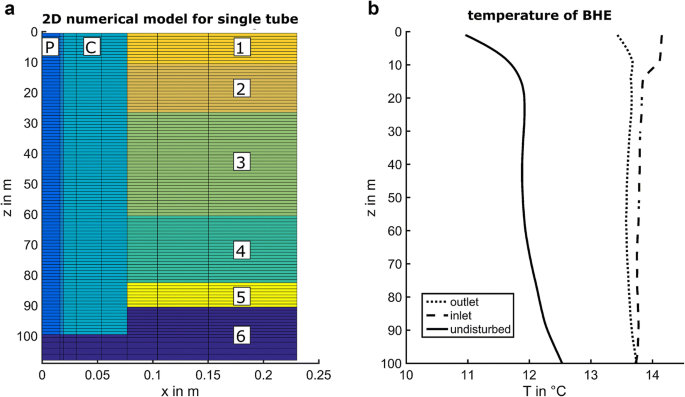

  

  a 2D model of a BHE tube using cylindrical coordinates—the vertical symmetry axis is at x = 0. The colors denote units with different physical properties. For example, the inner pipe (P), the pipe walls and the BHE’s cement (C) (from left to right) are shown in blue colors between x = 0 and x = 0.07 m. Layers 1 to 6 denote different geological units with thermal conductivities of 1.89, 2.6, 2.83, 3.41, 2.97 and 3.4 W m⁻¹ K⁻¹, respectively. b The dashed and dotted black lines show the simulated temperatures at the outer surfaces of the inlet and outlet tubes, respectively. The solid black line shows the undisturbed temperature

• 2. For specific depths, we model the temperature distribution inside and in the vicinity of the BHE using a 2D numerical model of the BHE’s cross section and its surrounding soil and rock (Fig. 3a). The simulation results are subsequently compared to the temperatures measured by the TSM. To infer flow velocity and direction, we look for the minimum of the root mean square error between the measured temperatures and those simulated for different groundwater flows. In Horizontal BHE model section, we explain the horizontal BHE model in detail.

  Fig. 3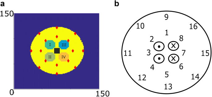

  

  Horizontal 2D model of the BHE (a) with color-coded domains and monitoring points marked in red. b Scheme of the TSM surrounding the BHE with numbered temperature sensors. The four circles in the middle show the inlet and outlet tubes marked by dots and crosses, respectively

Results and discussion

BHE pipe model

We are interested in the working fluid temperatures along the BHE inlet and outlet pipes. As the estimation of these temperatures is not trivial and analytical approaches even for U-tubes are complicated (Claesson and Javed 2018), we only consider a single pipe and make use of its cylindrical symmetry. Figure 2a shows the model in cylindrical coordinates with the axis of symmetry in the middle of the pipe. The model consists of the working fluid, the pipe wall, the BHE filling (cement) and the surrounding Earth layers. This model has 20 cells in the radial direction and 120 cells in the axial direction which corresponds to an overall radius of 2.5 m and a depth of 160 m. The cell size in the radial direction varies in relation to the BHE components from 16 mm to 1 m; in the axial direction, the cell size is 0.1 m. Table 1 gives additional information about the model, e.g., the pipe geometry and the thermal properties used. The thermal properties of the underground materials were taken from EGRT tests (Kappelmeyer 2011) and from geophysical laboratory measurements (Pechnig and Mottaghy 2012). The horizontal, colored bands, 1 to 6, in Fig. 2a represent the underground layers with thermal conductivities ranging from 2 to 3.4 W m⁻¹ K⁻¹. For the initial, undisturbed temperature distribution of the model, we use the temperatures measured by the DTS and from well logging data before BHE operation.

Table 1 Parameters for the simulation of the working fluid temperature along the BHE

We run two simulations. First, we simulate the temperature distribution for the inlet tube, i.e., for a downward flowing working fluid. As input, we use the BHE’s real inlet temperature and flow rate of 14.5 °C and 24.4 L/min, respectively. Subsequently, the calculated time-dependent fluid temperature at the bottom of the inlet pipe is used as input for the second simulation. Here, we simulate the temperature distribution of the outlet tube, i.e., for the upward streaming working fluid. We run both simulations until reaching steady-state conditions after approximately 4 h.

Figure 2b shows the calculated temperatures at the outer walls of the inflow and outflow pipes after 4 days of operation. In the first 10 m to 15 m below ground, both the inlet and outlet temperatures decrease considerably because of the low temperatures in this region. They are influenced by the previous winter, i.e., they are on average 5 K below the temperatures in deeper regions. Because of the initial and undisturbed seasonal underground temperature distribution, the inlet and outlet temperatures decrease considerably. Below this, both temperatures remain more or less constant; they only vary in a range of ± 0.15 K. The temperature differences between the inlet and outlet pipes decrease with depth. From the simulations, we deduce the pipe wall temperatures at the TSM positions. At 82 m depth, they are 13.8 °C and 13.7 °C, and at 94 m, they are 13.8 °C and 13.75 °C for the inlet and outlet pipes, respectively.

The introduced model and the simulation sequence simplify the BHE and neglect the interaction between the inlet and outlet pipes. However, neglecting the horizontal heat flow seems reasonable because of the small temperature differences between the pipes. Moreover, the simulated temperatures agree with the DTS measurements recorded for the last 30 m along the BHE as shown in Results of TSMs section. Therefore, we conclude that we can approximate the temperature distribution along the inlet and outlet pipes with the introduced approach at least for short BHE operation periods. We use the calculated inlet and outlet tube temperatures at the TSM positions as input for the horizontal BHE model discussed in the next section.

Horizontal BHE model

We apply the model, which we introduce here, to study the influence of groundwater flow on the temperature distributions recorded by the TSMs. With the model at hand, we study the sensitivity of the temperature distributions measured at the sensor positions to groundwater flow. The 2D model represents a horizontal cross section of a BHE and the surrounding soil (Fig. 3a). In Fig. 3a, b, the four inner circles represent the inlet and outlet tubes of the BHE. The square in the middle of Fig. 3a approximates a tube used to grout the cement into the BHE. Figure 3b shows the inner part of the model, i.e., a scheme of the TSM where the numbers represent the temperature sensors. The model consists of 75 by 75 cells with a cell size varying from 3.2 mm up to 8 cm at the outer boundaries, which corresponds to an area of 1 m × 1 m.

Using the parameters given in Table 2, we simulate temperature distributions for different groundwater flow scenarios. We vary the groundwater flow velocity from 4 × 10⁻⁶ m s⁻¹ down to zero flow (flow direction of 0°, i.e., from sensor 1 to 5, see Fig. 3b) and the flow direction from 0° to 337.5° in steps of 22.5° at a constant velocity of 3 × 10⁻⁶ m s⁻¹. Figure 4 summarizes the simulation results for the TSM at 82 m depth. In Fig. 4a, b, we show the temperatures for different incident angles at the inner and outer rings, respectively. At the inner ring, the variation in flow direction influences the temperature only slightly with a maximal temperature change of only 50 mK compared to the temperatures without groundwater flow. The temperatures of the inlet tubes and outlet tubes, even though they differ by only 0.1 K, dominate the temperature distributions measured on the inner ring. Therefore, the flow direction cannot be deduced from the inner ring data.

Table 2 Parameter of the horizontal BHE model

Fig. 4

Simulated temperatures at the TSM at 82 m depth. The left and right columns show the temperatures at the inner and outer ring sensors, respectively. In the upper row (a, c), the incident angle of the groundwater flow is varied, whereas the velocity is varied, for flow in the direction from sensor 6 to 2 in the lower row (b, d), which equals 247.5°

At the outer ring, the influence of flow direction on temperature is greater but is still below 0.2 K for a temperature difference between the working fluid and the ground of approximately 1.5 K. However, the flow direction affects the temperature distribution systematically (Fig. 4b). Thus, it can be deduced from the outer ring temperatures with a directional resolution of 22.5°.

A varying flow velocity similarly affects the TSM temperatures. While the temperature varies little at the inner ring, the velocity-dependent temperature changes are higher at the outer ring (Fig. 4c, d). Again, for the given temperature difference, they are approximately 0.2 K compared to the no flow conditions and are not very high. Therefore, considering the 50 mK standard deviation of the TSM sensors, only flow velocities above 10⁻⁶ m s⁻¹ can be resolved at a depth of 82 m.

We conclude from the sensitivity study that the inner sensor ring is essential to determine the position of the TSM relative to the BHE tubes. The temperatures of the inlet and outlet tubes dominate the temperatures measured at the inner ring, even though groundwater flow slightly influences them as well. We observe the opposite effect at the outer ring. Here, the influence of groundwater flow dominates the measured temperatures. Thus, they can be utilized for inferring groundwater flow velocity and direction.

Results of TSMs

We used the temperatures recorded before BHE operation (over a period of 20 min) to calibrate the TSM sensors. To ensure steady-state conditions, i.e., drying of the backfilling cement, we measured these temperatures 1 month after installing the BHE. For a nonoperating BHE, all TSM temperature sensors at a given depth must have the same temperature. Thus, we calibrated the TSM sensors using DTS measurements as well as the temperatures measured by a probe in a nearby groundwater well. At depths of 82 m and 94 m, the temperature is approximately 12 °C and 12.24 °C, respectively. For each sensor, a temperature offset was stored and used for correcting the temperature measurements during the experiment. We found the standard deviation of the sensors was less than 30 mK when averaging 12 measurements.

In Fig. 5, we show measured DTS temperatures of the last 30 m of the BHE before and during its operation. The DTS temperatures during BHE operation are also shown for steady-state conditions. Because the TSM’s casing contributes to the overall thermal conductivity at the location where it is mounted, it induces a temperature decrease at each installed location. While the temperature measured by the DTS increases over the entire BHE, locally at the TSM positions, the measured temperatures are smaller than expected in a single BHE. The TSM temperatures are shown at their expected positions by black squares. The DTS temperatures during BHE operation are higher (solid lines). However, they deviate slightly from the TSM temperatures as the DTS cables were mounted outside of the TSM modules. Therefore, the DTS temperatures at the TSM positions have local minima at approximately 82 m and 94 m, where we expect the TSM, i.e., the DTS data confirm the TSM positions.

Fig. 5

Temperatures measured 70 m to 100 m below the surface before and during BHE operation. The dashed lines show the temperatures measured with the DTS method before BHE operation and with a temperature probe in a nearby well (without BHE). The black squares show the TSM temperatures before BHE operation. The solid lines show the temperatures measured by DTS during BHE operation

In addition to the TSM depths, the TSM orientation is required for deducing the groundwater flow direction. For the TSM orientation, we use the magnetic field sensors (HCM5885) of the TSM. First, we calibrated each TSM with respect to the Earth’s magnetic field at the investigation site. Subsequently, we monitored the magnetic field data during installation and BHE operation. Figure 6 shows the TSM direction relative to the Earth’s magnetic field for both TSMs (Fig. 6a in 82 m and Fig. 6b in 94 m) during and shortly after installation. It seems that the magnetic field sensor of the TSM at 82 m had an aberration during the first operational interval. As natural torsion would cause a smoother change in orientation, we assume that the outliers measuring 90° are caused by electronic interference. In contrast, the magnetic field sensor of the TSM at 94 m shows a quite stable orientation of approximately (330 ± 1)°. We conclude that there is only negligible torsion of the modules during installation. Thus, the final TSM orientations correspond those at insertion of the TSMs into the drilling hole.

Fig. 6

TSM orientation recorded by magnetic field sensors for the TSM at 82 m and 94 m depth during installation

To validate the introduced methodology for determining groundwater flow and direction, we operated the testbed BHE for 14 days. During BHE operation, TSM data were collected every minute. Additionally, we recorded operational BHE data. These data remained nearly constant during BHE operation; flow rate, inlet and outlet temperature were 24 L min⁻¹, 14.5 °C and 14.1 °C, respectively. Both temperatures have an accuracy of 0.1 K. For analyzing the influence of groundwater flow on the temperatures measured by the TSM, we used the data recorded steady-state conditions. They were attained after 10 days of BHE operation. We selected a period with minimal variations of the inlet and outlet temperatures. As described in BHE pipe model section, they are used for simulating the fluid temperatures of the inlet and outlet tubes at the BHE depths.

We present the TSM data together with the numerical simulation results at depths of 82 m and 94 m in Figs. 7 and 8, respectively. In both figures, subplots a and b show the temperatures of the inner and outer rings before BHE operation, and subplots c and d show the steady-state temperatures of the inner and outer rings during BHE operation, respectively. The dashed black lines show the numerical simulations for no flow conditions, while the solid black lines show the numerically calculated temperatures at the sensor positions with groundwater flow. The black squares depict the measured temperatures with their standard deviations shown as error bars. Additionally, we summarized the measured and simulated data for the inner and outer rings in subplots (polar plots) e and f, respectively.

Fig. 7

Measured and simulated TSM temperatures at 82 m depth. The left and right columns show the inner and outer ring temperatures, respectively. They are shown both as a standard plot (a–d) and as a polar plot (e, f). a, b show the temperatures before BHE operation, c, d the steady-state temperatures during BHE operation. Black squares represent the measured data; solid and dashed black lines represent the simulated temperatures with and without groundwater flow, respectively. The red square marks the position of the first sensor

Fig. 8

Measured and simulated TSM temperatures at 94 m depth. The left and right columns show the inner and outer ring temperatures, respectively. They are shown both as a standard plot (a–d) and as a polar plot (e, f). a and b show the temperatures before BHE operation, c and d the steady-state temperatures during BHE operation. Black squares represent the measured data; solid and dashed black lines represent the simulated temperatures with and without groundwater flow, respectively. The red square marks the position of the first sensor

At a depth of 82 m, the mean temperature before BHE operation is approximately 12 °C for all sensors (Fig. 7a, e). At BHE operation, one can identify the sensor positions at the inner ring with respect to the inlet and outlet tubes (Fig. 7e); sensors 1 and 3 are close to the inlet tubes, while sensors 5 and 7 are next to the outlet tubes. The influence of groundwater flow on the temperature distribution is best seen in the outer ring sensors (Fig. 7d, f). They prove that groundwater flow has to be taken into account to reproduce the observed temperatures in the simulation. For different scenarios with various groundwater flow directions and gradual increasing flow velocities ranging from 0.4 × 10⁻⁶ m s⁻¹ to 4.5 × 10⁻⁶ m s⁻¹, we numerically computed the temperatures at the TSM sensor positions. Subsequently, we compared them with the measured temperatures. The minimal root mean square error between the measured and calculated temperatures is found for a groundwater flow velocity of approximately 4 × 10⁻⁶ m s⁻¹ in the NW direction at 82 m depth.

For data interpretation, various error sources must be considered. In addition to the errors of the temperature sensors, their positions can change during installation. This would cause a deviation between the predicted and measured temperatures. Additionally, the TSM casing and electronic parts are not considered in the simulation, which might result in a slight deviation as well. However, this error is negligible under steady-state conditions.

Analogous to Fig. 7, Fig. 8 shows the measured and calculated temperatures at a depth of 94 m. Again, the positions of the inlet and outlet tubes relative to the TSM can be deduced from the inner ring temperatures (Fig. 8e). As the warmer working fluid flows into the inlet tubes, the sensors close to them show higher temperatures. Inner ring sensor 1 as well as the outer ring sensors 9 and 16, which outrange the predicted temperatures, must be considered with caution. We assume that a displacement of the sensors during installation caused this deviation. As their initial temperatures are consistent with the other sensors, they seem to work properly.

For the TSM at a depth of 82 m, we compare the measured and simulated data of the outer TSM ring at 94 m (Fig. 8d, f) to infer groundwater flow. The temperature difference between the measured and the simulated data without groundwater flow is below the 50 mK standard deviation of the temperature sensors. Thus, no groundwater flow above the resolution limit of 8 × 10⁻⁷ m s⁻¹ can be identified at a depth of 94 m. However, we found the lowest root mean square error between the measured and calculated temperatures (with flow) for a groundwater flow velocity of 2 × 10⁻⁷ m s⁻¹ in SW direction (solid black line in Fig. 8f).

For comparison, we measured groundwater flow using a commercially available optical measurement tool developed by PhreaLog (Schöttler 2000). With the optical measurement probe, particle trajectories within the groundwater can be detected in an observation well. Thus, groundwater flow direction and velocity can be derived from a time series of particle trajectories images. The measurements were taken in a nearby well at different depths. At 82 m, we measured a flow rate of 3 × 10⁻⁵ m s⁻¹ in the NW direction. While the direction matches the TSM result, the velocity determined with the optical tool is one order of magnitude higher. The difference in velocity may be caused by horizontal permeability variations or, more likely, by the measuring principle of the optical tool. It measures water flow in an open water well, i.e., the natural flow is disturbed by the missing rock matrix. Thus, measured flow velocities must be considered higher than the real groundwater flow velocity (Freeze and Cherry 1979). The velocities measured by the optical tool probe in the observation well spread in a width range depending on the depth. Reasons for this apart from the different permeability of the layers, i.e., due to backfilling filtering materials surrounding the well or special casing inlets inside the well, can be also vertical flow of groundwater due to lowering or raising the tool. In principle, the change in the flow potential and the permeability changes listed in the sentence above mean that the calculation of the actual groundwater flow velocity can be complex. The filter velocity inside the well must be converted into the groundwater flow velocity in the aquifer. Those side-effects are nonexistent when estimating groundwater flow velocities of BHEs equipped with TSMs. Due to the direct contact between TSMs and the rock matrix, the temperature measurements are not affected by unwanted physical mechanisms.

Moreover, in groundwater protection areas, a TSM could be also applied for BHE leakage monitoring. In the case of a BHE leakage, the center temperature sensors next to the point of leakage would register an abrupt temperature change. However, TSMs would only detect leakages close to their vertical positions. They would not register BHE leakages at other depths.

Finally, yet importantly, we would like to touch on the economic aspect in the discussion. We cannot yet provide a cost for the TSM, but the investment cost for many TSMs would be small in comparison with the cost of a BHE or even a BHE field. The operational costs are negligible due to the passive operation, i.e., TSM sensors can automatically record temperatures at any desired sampling rate and period.

Conclusions and outlook

We present a successful test of the novel temperature sensor module (TSM) for measuring groundwater flow. The TSM works passively by measuring the temperature distribution inside and within the direct vicinity of a BHE. The temperature distribution allows determination of advective heat transport and hence groundwater flow. As a testbed system, we installed two TSMs at a BHE at depths of 82 m and 94 m. At a depth of 82 m, we found groundwater flowing in a NW direction with a velocity of approximately 4 × 10⁻⁶ m s⁻¹, which corresponds to a speed of 0.35 m/day. At 94 m depth, groundwater flow is below the resolution limit, i.e., the temperature change due to advective heat transport is less than 50 mK, the standard deviation of the temperature sensor. However, the groundwater flow resolution of the TSM depends on the temperature difference between the underground materials and the BHE. Therefore, by increasing the temperature difference between the working fluid and the subsurface, which can be achieved by increasing the heating or cooling power for the BHE fluid or its flow rate, the resolution of the groundwater flow velocity can be increased.

We also compared the groundwater flow measured with the TSM with a commercially usable optical measurement method for groundwater wells. The result showed agreement in the determination of the groundwater flow direction. The groundwater flow velocity deviated by about one order of magnitude due to the different geometry and material conditions, but this is also to be expected.

So far, we only discussed only the one-time determination of groundwater flow with the TSM. However, when installed on a BHE, a TSM can monitor temperatures over long periods. Thus, they can provide data on the long-term behavior of the BHE and/or groundwater flow. For example, they could detect seasonal variations in groundwater flow, changes in the thermal properties of the BHE filling or changes in the thermal resistance between the BHE and the ground. Thus, a BHE equipped with multiple TSMs would provide long-term information, which is otherwise not available, for optimizing the operation of the corresponding geothermal field.

References

ADT7240 Datasheet. Analog devices, digital temperature sensors. 2019. http://www.analog.com/media/en/technical-documentation/data-sheets/ADT7420.pdf. Accessed 01 May 2019.
Alberti L, Angelotti A, Antelmi M, LaLicata I. A numerical study on the impact of grouting material on borehole heat exchangers performance in aquifers. Energies. 2017. https://doi.org/10.3390/en10050703.
Carslaw HS, Jaeger JC. Conduction of heat in solids. 2nd ed. Oxford: Oxford University Press; 1959.
Claesson J, Eskilson P. Conductive heat extraction to a deep borehole: thermal analyses and dimensioning rules. Energy. 1988;13(1988):509–27.
Claesson J, Javed S. Explicit multipole formulas for calculating thermal resistance of single U-tube ground heat exchangers. Energies. 2018;11:214. https://doi.org/10.3390/en11010214.
Clauser C. Numerical simulation of reactive flow in hot aquifers. SHEMAT and processing SHEMAT. Heidelberg: Springer; 2003.
de Palya M, Hecht-Méndez J, Beck M, Blum P, Zell A, Bayer P. Optimization of energy extraction for closed shallow geothermal systems using. Geothermics. 2012;43:57–65.
Deutsche Gesellschaft Für Geotechnik E.V. Shallow geothermal systems: recommendations on design, construction, operation and monitoring. Berlin: Wilhelm Ernst & Sohn; 2016. https://doi.org/10.1002/9783433606674.
Diao N, Li Q, Fang Z. Heat transfer in ground heat exchangers with groundwater advection. Int J Therm Sci. 2004;43(12):1203–11.
Freeze RA, Cherry JA. Groundwater. London: Prentice Hall, International Inc.; 1979.
Fütterer J, Constantin A. Energy concept for the E.ON ERC main building. 49th ed. Aachen: E.ON Energy Research Center; 2014.
Fütterer J, Constantin A, Müller D. An energy concept for multifunctional buildings with geothermal energy and photovoltaic. In: Proceedings CISBAT (Cleantech for sustainable buildings from nano to urban scale) 2011. Lausanne: Ecole Polytechnique Fédérale de Lausanne; 2011. p. 697–702.
GTC Kappelmeyer GmbH. Enhance geothermal response test, EGRT—RWTH E.ON Energy Research Center, Faseroptische Temperaturmessungen, Bericht, unveröffentlicht. Karlsruhe: GTC GmbH; 2011.
Guaraglia DO, Pousa JL. Introduction to modern instrumentation for hydraulics and environmental sciences. Berlin: Walter de Gruyter GmbH & Co; 2014. ISBN 978-3-11-040172-1.
He H, Dyck MF, Horton R, Li M, Jin H, Si B. Distributed temperature sensing for soil physical measurements and its similarity to heat pulse method. Adv Agron. 2018. https://doi.org/10.1016/bs.agron.2017.11.003.
Hecht-Mendez J, de Paly M, Beck M, Bayer P. Optimization of energy extraction for vertical closed—loop geothermal systems considering groundwater flow. Energy Convers Manage. 2013;66:1–10.
Hellström G. Comparison between theoretical models and field experiments for ground heat systems. In: International conference on subsurface heat storage in theory and practice. 1983, pp. 102–15.
HMC5883L Datasheet. Farnell. 2019. http://www.farnell.com/datasheets/1683374.pdf. Accessed 01 May 2019.
Luo J, Rohn J, Bayer M, Priess A. Thermal efficiency comparison of borehole heat exchangers with different drillhole diameters. Energies. 2013;6:4187–206. https://doi.org/10.3390/en6084187.
Michalski A, Klitzsch N. Temperatursensormodul für Grundwasserströmungen. German Patent DE102016203865. 2017.
Michalski A, Klitzsch N. Temperature Sensor Module for Groundwater flow detection around borehole heat exchangers. Geotherm Energy Sci Soc Technol. 2018;6:15. https://doi.org/10.1186/s40517-018-0101-8.
Morgenstern A. Entwicklung einer Einbohrloch-Messsonde zur Bestimmung der horizontalen Fließparameter ohne Störung des Strömungsfeldes, Dissertation, Technische Universität Cottbus; 2005.
Omer AM. Ground-source heat pumps systems and applications. Renew Sust Energy Rev. 2008;12:344–71.
Pechnig R, Mottaghy D. Erstellung und Kalibrierung eines numerischen geothermischen Modells für das E.ON ERC Erdwärmesondenfeld. Aachen: Erläuterungsbericht der Geophysica Beratungsgesellschaft mbH; 2012.
Rath V, Wolf A, Bücker M. Joint three-dimensional inversion of coupled groundwater flow and heat transfer based on automatic differentiation: sensitivity calculation, verification, and synthetic example. Geophys J Int. 2006;167:453–66.
Riveraa JA, Blum P, Bayera P. Analytical simulation of groundwater flow and land surface effects on thermal plumes of borehole heat exchangers. Appl Energy. 2015;146(15):421–33.
Schöttler M. Informationen zum GFV-Messsystem. Firmenschrift. 2000. http://www.phrealog.de/images/MediaCenter/PHREALOG_Horizontale_Fliessmessung.pdf. Accessed 2 Dec 2019.
Schöttler M. Erfassung der Grundwasserströmung mittels des GFV-Messsystems. Geotechnik. 2004;27:41–6
Acknowledgements
The authors are thankful for the financial support of the German Federal Ministry of Economics and Energy-funded project “exegetically optimized HVAC control with dynamic and flexible integration of a monitored geothermal borehole heat exchanger field” under Grant 03ET1022A.
Funding
This work is funded by the German Federal Ministry of Economics and Energy (BMWi) under the Grant (Bundesministerium für Wirtschaft und Energie) 03ET1022A.
Author information
Authors and Affiliations
Contributions
Both authors contributed according to their respective areas of expertise. AM designed and constructed the temperature sensor module. He set up the numerical models and performed the numerical simulation. He also oversaw the drilling and installation of the BHE and TSM and performed the experiments. NK suggested the measuring method and helped analyzing the results. He drafted parts of the manuscript. Both authors read and approved the final manuscript.
Corresponding author
Ethics declarations
Ethics approval and consent to participate
Not applicable.
Consent for publication
Competing interests
The authors declare that they have no competing interests.
Additional information
Publisher's Note
Springer Nature remains neutral with regard to jurisdictional claims in published maps and institutional affiliations.
Rights and permissions
Open Access This article is distributed under the terms of the Creative Commons Attribution 4.0 International License (http://creativecommons.org/licenses/by/4.0/), which permits unrestricted use, distribution, and reproduction in any medium, provided you give appropriate credit to the original author(s) and the source, provide a link to the Creative Commons license, and indicate if changes were made.
About this article
Cite this article
Michalski, A., Klitzsch, N. First field application of temperature sensor modules for groundwater flow detection near borehole heat exchanger. Geotherm Energy 7, 37 (2019). https://doi.org/10.1186/s40517-019-0152-5
Received:
Accepted:
Published:
DOI: https://doi.org/10.1186/s40517-019-0152-5