GEOPHIRES v2.0: updated geothermal techno-economic simulation tool

Abstract

This paper presents a new version (v2.0) of the geothermal techno-economic simulation tool GEOPHIRES [GEOthermal energy for Production of Heat and electricity (“IR”) Economically Simulated]. GEOPHIRES combines reservoir, wellbore, and surface plant technical models with cost correlations and levelized cost models to estimate the capital and operation and maintenance costs, instantaneous and lifetime energy production, and overall levelized cost of energy of a geothermal plant. In addition to electricity generation, direct-use heat applications and combined heat and power or cogeneration can be modeled. Various upgrades have been implemented to develop GEOPHIRES v2.0, including: updating the built-in cost correlations, coupling to the external reservoir simulator TOUGH2, enhancing the built-in wellbore simulator, converting the programming language to Python, and making the code open-source. Users are encouraged to build upon the tool, e.g., by implementing their own correlations or coupling to other simulators. In this paper, we discuss the GEOPHIRES v2.0 objectives and history, and we present the software architecture as well as built-in models and correlations. We include two example simulations and quick-start guide on how to run a simulation.

Introduction

GEOPHIRES is a computer code to perform techno-economic simulations of geothermal energy systems. For a given set of input parameters, the tool simulates the subsurface reservoir, wellbore, and surface plant either by using built-in or external user-provided models. The simulated output includes the reservoir production temperature and instantaneous and lifetime surface plant heat and/or electricity production. Combined with capital and operation and maintenance (O&M) cost correlations, GEOPHIRES applies levelized cost models to estimate the overall required investment and levelized cost of electricity and/or heat (LCOE and LCOH). Possible end-use configurations are direct-use heat (e.g., for district heating or an industrial process), electricity, and cogeneration or combined heat and power (CHP). Ground-source heat pumps are not considered. The name GEOPHIRES is an acronym that stands for GEOthermal energy for Production of Heat and electricity (“IR”) Economically Simulated, with “IR” representing electric current and resistance and referring to the electricity mode.

The original version of GEOPHIRES (v1.0) was developed by one of the authors during the period 2012–2014 (Beckers et al. 2013, 2014). GEOPHIRES v1.0 was originally applied to assess the technical and economic performance of fracture-based enhanced geothermal systems (EGS) for electricity and direct-use heat applications. The capability to model matrix flow reservoirs was limited, and users could not alter the code to implement their own applications or couple to stand-alone models. To address these limitations, as well as to update the cost correlations, improve code readability, and add several new modeling features, a new version (v2.0) has been developed during the period 2017–2018. GEOPHIRES v2.0 is distributed as open-source under the permissive MIT license, i.e., others can build upon the framework for commercial and non-commercial purposes. A conference paper by Beckers and McCabe (2018) reported initial progress on the development of GEOPHIRES v2.0. This paper discusses in detail the overall model structure; built-in technical and cost correlations and sub-models; as well as options to couple to external simulators and implement user-provided code. We present two example simulations: the first one models a direct-use heat application with TOUGH2 (Transport of Unsaturated Groundwater and Heat v2) as an external reservoir simulator; the second example considers a hydrothermal reservoir for electricity production using an organic Rankine cycle (ORC) power plant.

Objective of GEOPHIRES v2.0

GEOPHIRES v2.0 has been designed to be a flexible, user-friendly, and robust computer tool for assessing technical and/or economic performance of a geothermal system with a wide possible level of simulation detail. By relying on built-in correlations and default values, a basic simulation can be performed with limited knowledge on subsurface, surface plant, and financing conditions. A more-experienced or knowledgeable user can perform a more in-depth analysis, e.g., by making use of the integration with the external reservoir simulator TOUGH2, or hard-coding in a specific surface plant application. The tool has built-in checks on each input parameter to ensure that the case modeled is realistic. A user guide and example cases are available to help a new user get familiar with the tool. Examples of cases that can be simulated with GEOPHIRES v2.0 are: investigating the payback period of a newly constructed geothermal power plant, sizing a geothermal district-heating system, assessing the impact of subsurface uncertainty (e.g., reservoir permeability, volume, and temperature) on overall geothermal plant performance, comparing different geothermal reservoir management strategies, estimating future electricity production using historical reservoir and plant operational data, and predicting the impact on future revenue of a system upgrade (e.g., drilling a new well or stimulating the reservoir).

Several analytical and numerical models have been developed to simulate specific components of a geothermal system (e.g., the reservoir or power plant); however, few tools exist that can perform an entire techno-economic simulation like GEOPHIRES. Advanced stand-alone reservoir simulators are plentiful, e.g., TOUGH2 (Pruess et al. 1999), FEFLOW (Diersch 2013), and CMG STARS (Computer Modeling Group Ltd 2007). These simulators can estimate the geothermal reservoir production temperature, but they need to be coupled to other models to calculate electricity production or investment cost. In GEOPHIRES, there are three different options for the reservoir component: the user can (1) import the temperature output of any reservoir simulator, (2) directly call TOUGH2, or (3) use one of the built-analytical models, as discussed in “Implementation” section. Various tools also exist to simulate the surface equipment, e.g., Tech Aspen (2009) and IPSEPro (SimTech 2003). These tools can be used to calculate the electricity production of a geothermal plant or the efficiency of a geothermal district-heating system. In GEOPHIRES, the user can import the performance calculations developed with these models or rely on built-in surface–plant correlations (see “Implementation” section).

Apart from GEOPHIRES, few tools exist that incorporate all the geothermal system components necessary to perform a full techno-economic simulation. Examples are the Geothermal Energy Technology Evaluation Model (GETEM) (DOE 2016), the Hot Dry Rock economic (HDRec) model (Heidinger et al. 2006) and the upgraded version Euronaut (Heidinger 2010), and the DoubletCalc model (Van Wees et al. 2012). While GEOPHIRES can model various end-use options (electricity, direct-use heat, cogeneration), GETEM, HDRec, and Euronaut only model electricity generation, and DoubletCalc is designed to simulate direct-use heat applications. Further, GEOPHIRES v2.0 can model any type of geothermal reservoir and be coupled to external simulators. HDRec and Euronaut only simulate fracture-based EGS reservoirs, DoubletCalc calculates doublet flow in matrix flow-permeable reservoirs, and GETEM represents the reservoir solely with a user-provided hydraulic and thermal drawdown parameter. Only GEOPHIRES and DoubletCalc are open-source, allowing other researchers to expand upon the tool.

History of GEOPHIRES

The software tool GEOPHIRES has evolved out of previous research and models that date back to the Fenton Hill Hot Dry Rock (HDR) project at Los Alamos National Laboratory (Tester et al. 1979). The work in that project resulted in the techno-economic HDR model, which was presented in detail in “Heat Mining” by Armstead and Tester (1987). In the late 1980s, this model was updated to the MIT-HDR model (Tester and Herzog 1990), and in the 1990s, a Windows user interface was developed to make the tool more accessible to the geothermal community (Kitsou et al. 2000). That model became known as the MIT-EGS model and was used in the “Future of Geothermal Energy” study (Tester et al. 2006).

From 2012 to 2014, the MIT-EGS model was modified extensively by Beckers and other members of the Tester research group at Cornell University to develop GEOPHIRES v1.0. In addition to incorporating different end uses beyond electricity production (direct-use heat and cogeneration), the built-in capital and O&M cost correlations were updated and a new levelized cost model (standard discounted levelized cost model), reservoir model (percentage thermal drawdown model), and wellbore model (Ramey’s heat transmission model) were implemented. Also, new heat-to-electricity conversion efficiency correlations for binary cycle (subcritical and supercritical) and flash (single and double) power plants were incorporated based on simulations in Aspen Plus (Tech Aspen 2009) and MATLAB (MathWorks 2012). GEOPHIRES v1.0 was introduced at the Stanford Geothermal Workshop (Beckers et al. 2013) and later described in detail in a journal article (Beckers et al. 2014) and dissertation (Beckers 2016). Various simulation examples are included in these papers. Other case studies using GEOPHIRES v1.0 include an analysis of the potential for deep geothermal district heating in New York and Pennsylvania (Reber et al. 2014) and at Cornell University (Tester et al. 2015), and an assessment of a hybrid geothermal–biomass cogeneration system for Cornell University (Beckers et al. 2015). During the period 2017–2018, major upgrades were implemented to develop GEOPHIRES v2.0, with details and results presented in this paper. These upgrades include converting the source code from FORTRAN to Python, making the tool open-source, updating the cost correlations, enhancing the wellbore simulator, and directly coupling it to the external reservoir simulator TOUGH2.

Implementation

This section presents the GEOPHIRES software architecture, built-in correlations and models, and options for the user to integrate their own models. Additional information is provided in the user manual located in the GEOPHIRES GitHub project folder.

Software architecture

The GEOPHIRES software architecture is illustrated in Fig. 1. The green rectangles are GEOPHIRES model components, the orange rectangles refer to user interface components, and the blue rectangle refers to the external reservoir simulator TOUGH2. Rectangles with a solid outline are always executed during a simulation run; rectangles with a dashed outline refer to optional or user-provided components. When running a simulation, GEOPHIRES executes the following components in consecutive order:

Fig. 1

GEOPHIRES software architecture. Green, orange, and blue rectangles refer, respectively, to internal GEOPHIRES components, external user interface components, and the external reservoir simulator TOUGH2

• 1. Importing and validation of user-provided input data If a necessary parameter is missing, GEOPHIRES outputs a warning message and assumes a default value. Allowable value ranges for each parameter are included in the user manual.

• 2. Reservoir simulation GEOPHIRES calculates the production temperature over time either by using one of the built-in reservoir models, importing an external user-provided temperature data file, or by running the external reservoir simulator TOUGH2.

• 3. Wellbore simulation GEOPHIRES estimates the geofluid temperature change and the production and injection well pumping power.

• 4. Surface plant simulation GEOPHIRES calculates the amount of gross and net electricity and/or direct-use heat produced.

• 5. Cost calculations GEOPHIRES estimates the capital and annual O&M costs using built-in cost correlations or user-provided cost numbers. All costs in GEOPHIRES are expressed in US dollars ($).

• 6. Techno-economic metric calculation GEOPHIRES calculates as a default the techno-economic metric LCOH or LCOE. The code can be modified easily to compute other metrics, e.g., payback time, net present value (NPV), and internal rate of return (IRR). All economic results in GEOPHIRES are expressed in US dollars ($) or cents (¢).

• 7. Printing of results and messages GEOPHIRES prints calculation results and warning and error messages to the console and a text file.

The GEOPHIRES input and output text files are self-explanatory, meaning that no other user interface tool is needed. However, users can provide their own user interface or master file, for example, to automate running batches of simulations or to visualize GEOPHIRES results.

Built-in models and correlations

End-use options

Five different end-use options are available in GEOPHIRES:

• 1. Electricity All produced geothermal fluid is used to generate electricity with either an ORC or flash power plant.

• 2. Direct-use heat All produced geothermal fluid is used to provide heating for a given application, e.g., a district-heating system or industrial process.

• 3. Cogeneration or combined heat and power (CHP) Both heat and electricity are produced. Three different cogeneration configurations are available:

  • a. Cogeneration topping cycle A power plant is followed by a direct-use heat application in series. Heat at high temperatures from the geothermal fluid is first converted into electricity. Any remaining heat in the geothermal fluid after leaving the power plant is supplied to a low-temperature direct-use heat application.

  • b. Cogeneration bottoming cycle A direct-use heat application is followed by a power plant in series. In this less common configuration, the geothermal fluid first serves a high-temperature direct-use heat application. Any remaining heat in the geothermal fluid after leaving the direct-use heat process (at a user-specified temperature) is used to generate electricity. The heat-to-power conversion typically occurs with an ORC plant operating at low conversion efficiencies.

  • c. Cogeneration parallel cycle A power plant operates in parallel with a direct-use heat application. The produced geothermal fluid is split into two streams, providing heat at the same temperature to a power plant and direct-use heat application. The user specifies the fluid flow fraction going to each process.

Geofluid

The built-in fluid property correlations in GEOPHIRES for density, heat capacity, viscosity and vapor pressure are for pure water. However, these fluid property correlations are separate Python function in the open-source GEOPHIRES code which can easily be modified by the user for a different fluid, e.g., brine.

Reservoir models

Six reservoir models are available in GEOPHIRES to calculate the transient reservoir production temperature: (1) multiple parallel fractures model, (2) 1-dimensional linear heat sweep model, (3) m/A thermal drawdown parameter model, (4) percentage temperature drawdown model, (5) generic user-provided temperature profile, and (6) TOUGH2 reservoir simulator. The user specifies the reservoir model in the input file, and validation of relevant parameters is then performed to ensure compatibility of the selected model with the specified parameters. The output of the reservoir simulation component is a production temperature profile over the life of the project.

The first model—the Multiple Parallel Fractures Model (Gringarten et al. 1975)—is based on a linear model in which the reservoir is represented by an infinite series of parallel, equidistant, vertical fractures of uniform thickness. Due to the fracture-dominated nature of this model, it is intended primarily for EGS applications. In this model, heat transport occurs through thermal convection with 1-D water flow in the fractures and thermal conduction within the homogeneous, isotropic, and impermeable rock. The governing equations for the temperature of the rock and water in time and space are specified and solved in the Laplace domain and numerically converted back into the time domain. The dimensionless water temperature $T_{WD}$ (°C) is defined as:

$$ T_{W,D} = \frac{{T_{R,0} - T_{W} }}{{T_{R,0} - T_{{W,{\text{inlet}}}} }}, $$

(1)

with $T_{W,D}$ the water temperature (°C), $T_{R,0}$ the initial reservoir temperature (°C), and $T_{{W,{\text{inlet}}}}$ the water temperature at the reservoir inlet (°C). The full equation for the dimensionless temperature in Laplace space is given in Equation A17 in Gringarten et al. (1975). The model in GEOPHIRES is simplified by assuming that the temperature in the reservoir—and therefore, at the top and bottom of the fracture—is constant. With the simplification, the geothermal gradient is zero and the equation specifying the dimensionless water temperature in the Laplace space $\bar{T}_{W,D}$ is given as:

$$ \bar{T}_{W,D} \left( s \right) = \frac{1}{s}\exp \left( { - s^{1/2} \tanh \frac{{\rho_{W} c_{W} Qx_{E} }}{{2k_{r} H}}s^{1/2} } \right), $$

(2)

where $s$ is the Laplace variable (s⁻¹), $\rho_{W}$ is the density of the water (kg m⁻³), $c_{W}$ is the specific heat capacity of the water (J kg⁻¹ K⁻¹), $Q$ is the volumetric flow rate per fracture per unit depth of the fracture (m² s⁻¹), $x$ is the half-width fracture separation (m), $k_{r}$ is the rock thermal conductivity (W m⁻¹ K⁻¹), and $H$ is the height of the fractures (m). In GEOPHIRES v2.0, the conversion of this equation in Laplace space to the time domain is performed using the mpmath library (Johansson 2017).

The second model—the 1-Dimensional Linear Heat Sweep Model (Hunsbedt et al. 1984)—also focuses on modeling fractured geothermal reservoirs and therefore may be best suited for EGS applications. The model assumes that the reservoir can be represented as a porous medium with fluid surrounding blocks of rock characterized by a lumped effective rock radius. Heat transport in this model occurs through 1-D linear heat sweep of water through the reservoir. The dimensionless water temperature is defined as:

$$ T_{WD} = \frac{{T_{W} - T_{{W,{\text{inlet}}}} }}{{T_{R,0} - T_{{W , {\text{inlet}}}} }}. $$

(3)

The full equation for the dimensionless temperature in Laplace space is given in Eqs. 2–7a in Hunsbedt et al. (1984). This model in GEOPHIRES is simplified by setting the recharge temperature parameter to − ∞ (which specifies the fluid temperature at the reservoir inlet to remain constant over the lifetime instead of slowly increasing due to injection wellbore heat gains) and the external heat transfer parameter to zero (which specifies zero heat flux at the reservoir boundary). Both assumptions reflect a conservative modeling approach and are recommended by Hunsbedt et al. (1984) for unknown reservoir conditions. Thus, the equation specifying dimensionless temperature at the production well is given as:

$$ \bar{T}_{WD} \left( s \right) = \frac{1}{s}\left( {1 - \exp \left( { - Ks} \right)} \right), $$

(4)

where

$$ K = 1 + \frac{\text{NTU}}{{\gamma \left( {s + {\text{NTU}}} \right)}}. $$

(5)

NTU and $\gamma$ are the number of heat transfer units and the heat storage ratio, respectively. They are given as:

$$ {\text{NTU}} = \frac{{t_{\text{res}} }}{{\tau_{{{\text{ef}},r}} }} $$

(6)

and

$$ \gamma = \frac{{\rho_{W} c_{W} }}{{\rho_{r} c_{r} }}\frac{\phi }{1 - \phi }. $$

(7)

In these equations, $\phi$ is the rock porosity (–), $\rho_{r}$ is the rock density (kg m⁻³), $c_{r}$ is the rock specific heat capacity (J kg⁻¹ K⁻¹), $t_{\text{res}}$ is the residence time of water in the reservoir (s), and $\tau_{{{\text{ef}},r}}$ is the effective rock time constant (s), which is calculated as:

$$ \tau_{{{\text{ef}},r}} = \frac{{r_{{{\text{ef}},r}}^{2} }}{{3\alpha_{r} }}\left( {0.2 + \frac{1}{\it{Bi}}} \right) \left[ {\text{s}} \right]. $$

(8)

In this equation, $r_{{{\text{ef}},r}}$ is the effective rock radius representing the entire collection of rock blocks (m), $\alpha_{r}$ is the rock thermal diffusivity (m² s⁻¹), and ${\it{Bi}}$ is the Biot number (–). The value 0.2 represents the typical ratio of conduction path length to $r_{{{\text{ef}},r}}$ for spherical shapes (Hunsbedt et al. 1984). The effective rock radius and the Biot number are calculated as:

$$ r_{{{\text{ef}},r}} = 0.83\left( {\frac{3V}{4\pi }} \right)^{1/3} \,\,\,\,\,\,\,\left[ {\text{m}} \right] $$

(9)

and

$$ {\it{Bi}} = \frac{{h r_{{{\text{ef}},r}} }}{{k_{r} }}, $$

(10)

with $V$ being the mean volume of the rock block (m³) and $h$ being the rock surface heat transfer coefficient (W m⁻² K⁻¹). The factor 0.83 in Eq. (9) is the Kuo sphericity and represents the typical mean sphericity of a distribution of irregularly shaped rock blocks found in geothermal reservoirs (Hunsbedt et al. 1984). More information on default/assumed values for various parameters, including the heat transfer coefficient (h), was provided by Beckers (2016).

The third model—the m/A Thermal Drawdown Parameter Model—is discussed in detail by Armstead and Tester (1987). This model represents the reservoir as a single rectangular fracture of specified area with a uniform flow of fluid passing over the fracture surface. The mass loading parameter (m/A) is defined as the mass flow rate per unit area of a single side of the fracture (kg s⁻¹ m⁻²) and is provided by the user, along with other rock properties. The dimensionless temperature is defined and calculated as:

$$ T_{WD} = \frac{{T_{W} - T_{{W,{\text{inlet}}}} }}{{T_{R,0} - T_{{W,{\text{inlet}}}} }} = {\text{erf}}\left( {\frac{1}{m/A}\frac{1}{{c_{W} }}\sqrt {\frac{{k_{R} \rho_{R} c_{R} }}{t}} } \right), $$

(11)

where erf is the error function and $t$ is the time in seconds.

The fourth model—the Percentage Temperature Drawdown Model—expresses the thermal drawdown as a percentage temperature decrease per year. Previous iterations of this reservoir model used an exponential decline to model the drawdown over time. However, results from Snyder et al. (2017a) demonstrate that a linear decline with an annual temperature drop based on the percentage of the initial production temperature may fit measured production data more closely. Thus, the dimensionless temperature is defined and calculated as:

$$ T_{WD} = \frac{{T_{W} - T_{{W,{\text{inlet}}}} }}{{T_{R,0} - T_{{W,{\text{inlet}}}} }} = 1 - pt, $$

(12)

where $p$ is the percentage temperature decrease in units of years⁻¹ and t is the time in years.

The fifth model—the Generic User-Provided Temperature Profile—allows the user to specify and import a generic reservoir production temperature profile, with temperature data from an external simulation tool or measured data from an operating geothermal plant. The format for providing a generic temperature profile is via column vectors in a text file. An example case study using this reservoir model is included in the GEOPHIRES GitHub folder (example 2).

The sixth and final reservoir model—the TOUGH2 Geothermal Reservoir Simulator—is for nonisothermal multiphase flow in fractured porous media (Pruess et al. 1999). Its capabilities allow GEOPHIRES users a diverse set of options for modeling many types of subsurface conditions, including both matrix-dominated flow and/or fracture-dominated flow. In this GEOPHIRES reservoir model, the user either provides an external input file or uses a default input file and the TOUGH2 reservoir simulator is called within the Python code. The default input file is used when the user explicitly declares it or when the program is unable to find the user-specified input file in the working directory. The default model is a simple doublet case using a rectilinear permeable matrix reservoir structure and a single production and a single injection well. The production temperatures are taken directly from the TOUGH2 output files and processed to be compatible with the GEOPHIRES workflow. The user needs to have a license and executable for TOUGH2 to use this reservoir model.

The reservoir pressure drop is calculated by specifying an overall reservoir impedance, or productivity and injectivity index. When specifying a productivity and injectivity index, a reservoir hydrostatic pressure is either provided by the user or calculated using the built-in modified Xie–Bloomfield–Shook equation (DOE 2016). The reservoir pressure drop is combined with the wellbore pressure drop to estimate the pumping power, as discussed in “Wellbore model” section. While currently not implemented in GEOPHIRES, a third option to account for the reservoir pressure drop would be to directly import the pressure data from a TOUGH2 simulation.

Wellbore model

To account for production wellbore heat losses, the user can either specify a constant geofluid temperature drop or apply the built-in transient Ramey’s Wellbore Heat Transmission model (Ramey 1962) to estimate the geofluid temperature drop over time. Ramey’s model calculates the geofluid temperature drop in the production wells, $\Delta T_{\text{prod}}$, using the following equation:

$$ \Delta T_{\text{prod}} = \left( {T_{r,0} - T_{w} } \right) - \omega \left( {L - \varGamma } \right) + \left( {T_{w} - \omega \varGamma - T_{r,0} } \right){ \exp }\left( {\frac{L}{\varGamma }} \right)\,\,\,\left[ {^{ \circ } {\text{C}}} \right], $$

(13)

with $T_{r,0}$ as the initial rock temperature at the bottom of the well (°C), $T_{w}$ as the geofluid temperature at the bottom of the well (°C), $\omega$ as the average geothermal gradient (°C m⁻¹), and $L$ as the depth of the reservoir (m), equal to the length of the well assuming vertical wells. The parameter $\varGamma$ is calculated assuming that the thermal resistances of the casing and cement are negligible:

$$ \varGamma = \frac{{m_{\text{prod}} c_{w} f\left( t \right)}}{{2\pi k_{r} }}\,\,\left[ {\text{m}} \right], $$

(14)

with $m_{\text{prod}}$ as the production wellbore flow rate (kg s⁻¹) and $f\left( t \right)$ as the time function for a line heat source given by:

$$ f\left( t \right) = - { \log }\left( {\frac{{d_{\text{cas}} }}{{4\sqrt {\alpha_{r} t} }}} \right) - 0.29. $$

(15)

In this time function equation, $d_{\text{cas}}$ is the outer diameter of the casing (m). The time $t$ is the cumulative time that the well has been producing, i.e., by accounting for the utilization factor. Ramey’s model assumes the produced fluid is an incompressible, single-phase liquid with constant specific heat capacity. To calculate transient wellbore heat transmission for compressible or two-phase fluids, or to account for temperature and pressure dependency of fluid properties, a more advanced wellbore simulator should be implemented. To account for heat transmission in the injection wells, the user can specify a constant temperature gain. Ramey’s model has not been implemented for the injection wells because the built-in reservoir models (1 to 4) require a constant reservoir inlet temperature.

The injection and production well pumping power is estimated in GEOPHIRES by calculating the frictional and hydrostatic pressure drop in the well and the reservoir pressure drop. When the user opts to specify an overall reservoir impedance, the production and injection wells are assumed to be in hydraulic communication, the geofluid operates in a closed loop, and no flashing is allowed in the production wells or at the surface. In this case, the same approach for calculating the total pressure drop and pumping power is followed as in GEOPHIRES v1.0 (Beckers 2016). When specifying a productivity and injectivity index, the production and injection wells are treated individually following the same approach as GETEM (DOE 2016). The production wellhead pressure is provided by the user or set to 344.7 kPa (50 psi) above the water vapor pressure at production temperature (DOE 2016). When simulating a flash power plant, pumping of injection wells is considered but not of production wells, because the produced fluid is generally in two-phase flow. For ORC plants and direct-use heat applications, pumping of both injection and production wells is the default. Line-shaft pumps are considered for pumping of production wells with the necessary depth to prevent cavitation calculated by GEOPHIRES. A warning message is issued if this calculated depth is greater than 600 m.

GEOPHIRES calculates at each time step the frictional pressure drop in each well ($\Delta P_{\text{well,fr}}$) using the Darcy–Weisbach equation (Fox et al. 2004):

$$ \Delta P_{\text{well,fr}} = f\rho_{{w,{\text{well}}}} \frac{{v^{2} }}{2}\frac{L}{{d_{\text{well}} }}\,\, \left[ {\text{Pa}} \right], $$

(16)

with $f$ as the Darcy friction factor (−), $\rho_{{w,{\text{well}}}}$ as the temperature-averaged density of the water in each well (kg m⁻³), $v$ as the average water velocity in the well (m s⁻¹), and $d_{\text{well}}$ as the wellbore diameter (m). For turbulent flow, the Darcy friction factor is calculated using the Colebrook–White equation (Fox et al. 2004):

$$ \frac{1}{\sqrt f } = - 2 \cdot { \log }_{10} \left( {\frac{{{\raise0.7ex\hbox{$e$} \!\mathord{\left/ {\vphantom {e {d_{\text{well}} }}}\right.\kern-0pt} \!\lower0.7ex\hbox{${d_{\text{well}} }$}}}}{3.7} + \frac{2.51}{{{{Re}}\sqrt f }}} \right), $$

(17)

with $e$ as the wellbore pipe surface roughness (default set to 0.0001 m) and ${\it{Re}}$ as the Reynolds Number for flow in the wellbore ().

The hydrostatic pressure in each well $\Delta P_{\text{well,hydro}}$ is calculated as follows:

$$ \Delta P_{\text{well,hydro}} = \rho_{{w,{\text{well}}}} gL\,\, \left( {\text{Pa}} \right), $$

(18)

with g as the gravitational acceleration (9.81 m s⁻²). The difference in water density between production and injection well can cause a significant buoyancy effect that offsets some of the required pumping power. The water temperature profile along the well due to wellbore heat transmission causes a density profile along the wellbore. However, simulations using Ramey’s model show that, after a few months of operation, the water temperature difference between top and bottom of each well is typically less than 10 °C resulting in a density difference of only a few percent. This justifies considering a temperature-averaged water density for each well.

The built-in Ramey and frictional pressure drop models assume that all wells are vertical and of equal depth. In addition, all injection and production wells are assumed to have the same injection and production wellbore diameter, and the same injection and production fluid flow rate, respectively. The code can easily be modified to account for deviated and horizontal wells, as well as different diameters, depths, and flow rates for different wells. In case of non-vertical wells, the user should specify for each well the total vertical depth (TVD) along with a measured depth (MD). The bottom-hole temperature and hydrostatic pressure is calculated based on the TVD; frictional pressure drop loses and wellbore costs are based on the MD. The Ramey model should be deactivated for non-vertical wells, because that model is only valid for vertical wellbore geometry. Instead, a constant production wellbore temperature drop can be specified by the user to capture production wellbore heat losses. In case of wells with different diameters, depths, and/or flow rates, the user should calculate the frictional pressure drop, hydrostatic pressure, wellbore heat transfer, and well cost for each well individually and store the results in arrays. Pumping requirements should be evaluated for each well individually. The average production temperature can be calculated by lumping together the produced fluid from each well. The total well cost is calculated by adding up the well cost for each well.

Surface plant

If electricity is selected as the end-use product, then GEOPHIRES calculates the power production $P$ (MW_e) by multiplying the utilization efficiency of the power plant $\eta_{u}$ with the exergy of the produced geothermal fluid $B$:

$$ P = \eta_{u} B\,\,\,\, \left[ {{\text{MW}}_{\text{e}} } \right]. $$

(19)

The exergy is calculated based on the specific enthalpy $h$ (J kg⁻¹) and specific entropy $s$ (J kg⁻¹ K⁻¹) of the geothermal fluid at the production (prod) and ambient conditions (0):

$$ B = m_{\text{tot}} \left( {h_{\text{prod}} - h_{0} - T_{0} \left( {s_{\text{prod}} - s_{0} } \right)} \right)\,\, \left[ {\text{MW}} \right], $$

(20)

with $m_{\text{tot}}$ as the total mass flow rate produced (kg s⁻¹) and $T_{0}$ as the ambient temperature (K). GEOPHIRES has a built-in approximate correlation for calculating $B$ for pure water. Alternatively, steam tables or user-provided correlations can be used. Correlations for the utilization efficiency as a function of geothermal fluid production and ambient temperature were developed using power plant models in Aspen Plus and MATLAB for sub- and supercritical ORC and single- and double-flash power plants (Beckers 2016). The correlations are shown in Fig. 2 and have been implemented in GEOPHIRES. When selecting electricity or cogeneration as end-use, the user chooses as input one of these 4 power plant types. The ORCs are single-pressure, have air-cooled condensers, and a recuperator is included. No superheating is assumed in the subcritical cycle. Twenty-five refrigerants were evaluated and listed by Beckers (2016). The ORC correlations in Fig. 2 assume at each geofluid temperature, the refrigerant that maximizes the utilization efficiency is selected. For ambient temperatures different than 5 °C, 15 °C, or 25 °C, the utilization efficiency is linearly inter- or extrapolated. Explicit equations and a more detailed discussion on power plant specifications were provided by Beckers (2016). Correlations for the geothermal fluid temperature leaving the power plant were also developed and are incorporated in GEOPHIRES (Beckers 2016). These correlations are used in cogeneration mode with a topping cycle to estimate the geothermal fluid temperature available for a direct-use heat application. GEOPHIRES does not consider scaling (or mineral precipitation); however, scaling may put constraints on plant operating conditions, especially for hydrothermal reservoirs. For example, scaling of silica, caused by a decrease in geothermal fluid temperature, may put a lower limit on the injection temperature or require installing a chemical scale inhibitor system.

Fig. 2

GEOPHIRES built-in utilization efficiency correlations for ORC (subcritical and supercritical) and flash (single and double) power plants. Correlations provide power plant utilization efficiency as a function of production and ambient temperature

Various geothermal direct-use heat applications are possible, e.g., space and water heating, greenhouses, aquaculture, and industrial heat uses. GEOPHIRES does not have built-in correlations for these various applications to estimate plant performance and re-injection temperature as a function of production temperature, time of the day and year, etc. Rather, GEOPHIRES allows users to specify a utilization factor and thermal efficiency factor of the direct-use heat application, suitable for simple calculations. For more advanced representation of the surface plant, users are encouraged to implement their own correlations obtained, for example, from direct measurements or advanced process modeling simulations.

Cost correlations (capital and O&M)

The method in GEOPHIRES to estimate capital cost is based on the following: (1) capital cost consists of costs for exploration, drilling, surface plant, field gathering system, and reservoir stimulation, (2) built-in cost correlations incorporate indirect costs and contingency, (3) cost of financing is accounted for by the levelized cost model, and (4) capital cost escalation and debt on interest during construction is captured by a lumped capital cost multiplier. This method is similar to the method applied in the 2006 Future of Geothermal Energy Report (Tester et al. 2006) and the 1990 Heat Mining Report (Tester and Herzog 1990). The capital cost ($C_{\text{cap}}$) is calculated as follows:

$$ C_{\text{cap}} = C_{\text{wells}} + C_{\text{stim}} + C_{\text{gath}} + C_{\text{plant}} + C_{\text{expl}} \,\, \left[ {{\text{M}}\$ } \right], $$

(21)

with $C_{\text{wells}}$, $C_{\text{stim}}$, $C_{\text{gath}}$, $C_{\text{plant}}$, and $C_{\text{expl}}$ as the total well cost, reservoir stimulation cost, field gathering system cost, surface plant cost, and exploration cost, respectively. GEOPHIRES has built-in correlations for each of these capital cost terms. Users can use these correlations directly, multiply them by a factor, or provide their own cost figures. The built-in capital cost correlations are as follows:

• The total well cost ($C_{\text{wells}}$) is calculated as the cost per well multiplied by the user-provided number of production and injection wells. GEOPHIRES considers all wells to have the same depth; however, this assumption can easily be modified to account for various well depths. Four correlations are implemented to estimate the drilling and completion cost per well based on the work by Lowry et al. (2017). These correlations include 15% contingency and 5% for indirect costs (project management and engineering costs) (DOE 2016). These correlations are for small well diameter (0.16 m casing inner diameter) vs. large well diameter (0.22 m casing inner diameter), and vertical and open-hole vs. horizontal and with liner. They are plotted in Fig. 3. Correlation 4 falls within 10% of both the large diameter well cost correlation implemented in GETEM (DOE 2016) and the geothermal well cost correlation developed by Lukawski et al. (2014). Correlation 2 follows closely (within 10%) the small diameter well cost correlation in GETEM. GEOPHIRES assumes as default a 100% well drilling success rate, which may overstate actual field drilling success rates. Sanyal and Morrow (2012) found an average success rate of 71%, based on drilling and production data in 52 geothermal fields. GETEM assumes as default a 75% drilling success rate for hydrothermal development wells and 90% drilling success rate for EGS development wells. To account for failed wells in GEOPHIRES, the user can assign a drilling cost multiplier (e.g., a multiplier of 2 for a 50% drilling success rate).

  Fig. 3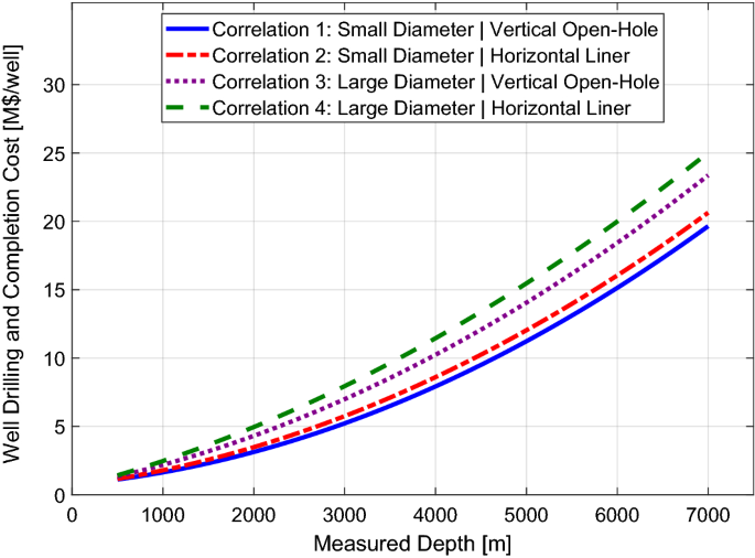

  

  GEOPHIRES built-in well drilling and completion cost correlations for four different well types (Lowry et al. 2017). Small and large diameter refers to 8½-in. and 12¼-in. bottom-hole diameter. Plotted cost data includes 15% contingency, but excludes indirect costs

• The built-in cost correlation for stimulating EGS-type reservoirs ($C_{\text{stim}}$) is $1.25 M per injection well (Beckers and Young 2017) plus 15% contingency and 5% for indirect costs (DOE 2016). For traditional hydrothermal reservoirs, this cost parameter is set to $0.

• The built-in cost correlation for estimating the field gathering system cost ($C_{\text{gath}}$) follows the same approach as GETEM (DOE 2016). $C_{\text{gath}}$ includes the cost for surface piping from each well to the plant and pumps for production and injection wells. The length of the surface piping is assumed 750 m per well at a cost of $500 per meter (DOE 2016). The pumping cost for each pump in the production wells (line-shaft pumps) and a single pump for the injection wells is calculated with the same correlation as GETEM (DOE 2016). An additional 15% is added for contingency and 12% for indirect costs (DOE 2016). $C_{\text{gath}}$ does not include the cost of pipelines to an off-site heat user or a district-heating system. These costs are estimated at $750 per meter pipeline length (Beckers and Young 2017) and can be manually added by the user to the pipeline distribution costs.

• The built-in power plant cost correlations ($C_{\text{plant}}$) are based on the original correlations developed by Beckers (2016), indexed to 2017 using the IHS Markit North American Power Capital Costs Index (NAPCCI) excluding nuclear plants (IHS 2018). The ORC power plant cost data have been updated with data from the 2016 GETEM tool (DOE 2016) and the geothermal binary power plants study by Verkís (2014). Figure 4 shows the power plant capital cost expressed in $ kW ⁻¹_e as a function of plant size and initial production temperature for subcritical ORC and double-flash power plants. The correlations in GEOPHIRES include 12% for indirect costs and 15% contingency. For the same plant size and production temperature, double-flash power plants are considered about 25% more expensive than single-flash power plants (Zeyghami 2010), and supercritical ORC plants are roughly 10% more than subcritical ORC plants (Astolfi et al. 2014). A wide range in power plant specific cost values is reported in academic and popular literature. The GEOPHIRES built-in surface plant cost correlations represent typical values. However, the user is recommended to provide their own power plant cost data if available for their case study. The ORC plant specific cost decreases only moderately at higher temperatures. The reasons are that when increasing the temperature, the ORC plant design also changes: (1) a different organic fluid is selected, (2) piping, pump, heat exchangers, and other equipment are designed to handle the higher temperature (and potentially also pressure), requiring thicker walls, potentially different materials, etc., and (3) additional components may be implemented, such as a heat recuperator, making the design and operation more complex. Unlike flash power plants, ORC plants are a small, niche market, typically case specific, and rely on relatively young technology, which has not been subject yet to decades of technological advancement. The cost for direct-use heat applications is highly dependent on the type of application. A generic cost of $250 kW ⁻¹_th plus 15% contingency and 12% indirect costs is assumed in GEOPHIRES. However, users are encouraged to provide their own cost figures for their specific application. Beckers and Young (2017) collected several cost figures to estimate the surface equipment cost for geothermal district-heating systems.

  Fig. 4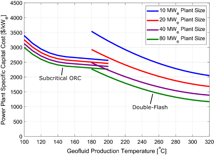

  

  GEOPHIRES built-in capital cost correlations for subcritical ORC and double-flash power plants. Plotted cost data includes 15% contingency, but excludes indirect costs

• The built-in exploration cost correlation ($C_{\text{expl}}$) considers drilling of a slim-hole well at 60% of the cost of a regular well, $1 M for geophysical and field work, an additional 12% on the total cost for technical and office support (indirect costs) and 15% for contingency (Beckers 2016).

This capital cost method is comparable to the method in GETEM with a few simplifications. GETEM considers a more detailed exploration, development and construction scheme where capital costs can be distributed over different years, and different discount rates can be assigned to different years. In GEOPHIRES, we consider the capital costs occur overnight and a lumped capital cost multiplier is available to capture effects such as capital cost escalation and debt on interest during construction. Further, unlike GETEM, GEOPHIRES does not consider capital costs for leasing, permitting and transmission lines. However, they could be manually added by the user as an additional capital cost term. While GEOPHIRES v1.0 only considered 15% contingency on drilling costs, all capital cost terms in GEOPHIRES v2.0 now consider 15% to align with more standard practices (as in GETEM). Similar to GETEM, no process contingency is considered in GEOPHIRES v2.0. However, if deemed applicable to a project, the user can manually account for process contingency by assigning a multiplier to the capital cost correlations (e.g., 1.2 for 20% process contingency).

GEOPHIRES estimates the annual O&M costs $C_{O\& M}$ (in M$ year⁻¹) as follows:

$$ C_{{{\text{O}}\&{\text{M}}}} = C_{{{\text{O}}\&{\text{M}},{\text{plant}}}} + C_{{{\text{O}}\&{\text{M}},{\text{wells}}}} + C_{{{\text{O}}\&{\text{M}},{\text{water}}}} + C_{{{\text{O}}\&{\text{M}},{\text{pump}}}} \,\,\,\,\,[{\text{M}}\$ {\text{ year}}^{ - 1} ], $$

(22)

with $C_{{{\text{O}}\&{\text{M, plant}}}}$, $C_{{{\text{O}}\&{\text{M,wells}}}}$, $C_{{{\text{O}}\&{\text{M,water}}}}$, and $C_{{{\text{O}}\&{\text{M, pump}}}}$ as the annual surface plant, wellfield, make-up water, and pumping O&M costs.

• GEOPHIRES estimates the annual surface plant O&M costs ($C_{{{\text{O}}\&{\text{M,plant}}}}$) as the sum of 1.5% of the total plant capital cost (for annual non-labor costs), and 75% of the annual labor costs, which is an approach similar to GETEM and GEOPHIRES v1.0 (Beckers 2016). The other 25% of the labor costs are assigned to the wellfield O&M cost. The labor costs are calculated internally in GEOPHIRES using the 2014 labor costs provided by Beckers (2016), indexed to 2017 using the Bureau of Labor Statistics (BLS) Employment Cost Index for utilities (BLS 2018). The original 2014 labor cost correlation expresses the labor costs as M$ year⁻¹ as a function of the plant size (MW) using an approximate logarithmic curve fit to the built-in labor cost data in GETEM (Beckers 2016).

• The built-in correlation for the wellfield O&M costs ($C_{{{{\text{O}}\&{\text{M,wells}}}}}$) is similar as the surface plant O&M costs: it assumes that $C_{{{{\text{O}}\&{\text{M,wells}}}}}$ consists of 1% of the total well plus field gathering system costs (for annual non-labor costs) and 25% of the labor costs (the other 75% of the labor cost were assigned to the surface plant O&M cost).

• To account for loss of water in the reservoir (especially in the case of EGS-type reservoirs), the user can provide a water loss rate. GEOPHIRES estimates the annual costs to buy make-up water ($C_{{{{\text{O}}\&{\text{M,water}}}}}$) using a water price of $3.5/1000 gallons.

• If the end-use option is direct-use heat only, then electricity is purchased at a user-provided electricity rate to power the geothermal fluid circulation pumps ($C_{{{{\text{O}}\&{\text{M,pump}}}}}$). In the case of electricity-only or cogeneration mode, the pumping power is considered auxiliary power and subtracted from the gross electricity generation.

Levelized cost models

GEOPHIRES v2.0 has three built-in models to calculate the levelized cost of energy: (1) the Fixed Charge Rate (FCR) model, (2) the Standard Levelized Cost model, and (3) the BICYCLE model. If the user selects electricity or cogeneration with electricity as the main product, then GEOPHIRES calculates the LCOE in units of ¢ kWh⁻¹. In the case of direct-use heat or cogeneration with direct-use heat as the main product, then GEOPHIRES calculates the LCOH in units of $ MMBtu⁻¹ (MMBtu = million Btu). The code can easily be modified to present the results in other units or to calculate other metrics such as NPV, IRR and payback period. However, these metrics, unit conversions, and necessary code modifications are not discussed in this paper.

The FCR model is the simplest levelized cost model, with the LCOE or LCOH calculated by (Armstead and Tester 1987):

(23)

with $C_{\text{cap}}$ as the total upfront capital investment (M$) and $C_{{\text{O}}\&{\text{M}}}$ as the average annual O&M cost (M$ year⁻¹; including cost for pumping power in direct-use heat mode). The parameter $R$ is used in the CHP mode and represents the average annual income from the secondary product (M$ year⁻¹), e.g., if electricity is the main product, then the levelized cost is calculated in LCOE, and $R$ is the secondary revenue from selling heat. The parameter $E$ is the average annual net amount of electricity or heat produced (kWh or MMBtu). The ${\text{FCR}}$ is a user-provided parameter and represents the fraction of total capital cost that must be paid each year (i.e., annuity) to pay off the total investment. It is based on the uniform capital recovery factor (UCRF), which depends on lifetime and discount rate, and tax rates, tax credits, insurance costs, depreciation, etc. (Short et al. 1995). Either a nominal levelized cost (current dollar analysis) or real levelized cost (constant dollar or “price year” dollar analysis) is calculated depending on whether the UCRF is based on a nominal or real discount rate (Short et al. 1995). Real discount rates exclude inflation whereas nominal discount rates include inflation.

The Standard Levelized Cost model discounts future revenue and expenditures to today’s dollars and calculates the levelized cost using the following equation (OECD/IEA 2015):

(24)

with $d$ as the real discount rate (−), ${\text{LT}}$ as the plant lifetime (years), and $C_{{{\text{O}}\&{\text{M}},t}}$, $E_{t}$, and $R_{t}$ as the O&M cost (M$ year⁻¹), energy production (kWh or MMBtu), and secondary CHP revenue stream (M$ year⁻¹), in year $t$, respectively. In Eq. (24), $C_{{{\text{O}}\&{\text{M}},t}}$ and $R_{t}$ are not corrected for inflation; therefore, $d$ is the real discount rate, and the levelized cost is calculated in constant dollars (Short et al. 1995). Alternatively, with a nominal discount rate in the denominator, the levelized cost is calculated in current dollars and accounts for inflation (Short et al. 1995). No taxes are considered in this levelized cost model.

The BICYCLE Levelized Life Cycle Cost model was developed at Los Alamos National Laboratory (Hardie 1981) and is the most detailed built-in levelized cost model in GEOPHIRES. It allows for accounting for variable debt/equity return rates, various tax rates (i.e., income, revenue, and property), and an investment tax credit (a tax credit as a percentage of the capital cost that is deducted from the income tax liability in the first year). All BICYCLE model equations implemented in GEOPHIRES were presented by Beckers (2016). The built-in version of the BICYCLE model requires as input the inflation rate and nominal discount rates (on equity and debt), and returns as output the real levelized cost in 2017 constant dollars. The BICYCLE model assumes linear depreciation of the invested capital over the plant lifetime with no salvage value.

All built-in cost correlations were either developed for 2017 constant dollars ($2017) or indexed from a previous year to $2017; therefore, the levelized cost results have the year 2017 as base year. Unlike for example GETEM, no cost index curves (e.g., for labor, wells, pumps, etc.) have been built-into convert the results into a different year. However, the user can either manually enter costs for a different year or implement their cost index correlations directly into the GEOPHIRES code.

Time stepping

GEOPHIRES assumes linear time discretization with a user-provided number of time steps per year over the lifetime of the plant. The default is four time steps per year, meaning a time step of 3 months. At every time step, GEOPHIRES calculates the reservoir output temperature, production wellhead temperature, direct-use heat and/or electricity power output (in MW), pressure drops and pumping power. On an annual basis, GEOPHIRES calculates the O&M costs and direct-use heat and/or electricity production (in GWh year⁻¹). To investigate seasonal effects, e.g., to assess the impact of more geothermal heat demand for district heating in winter than in summer, the user can select a smaller time step, e.g., a month (or 12 time steps per year). For even shorter timescale effects, e.g., to account for an hourly varying ambient temperature or investigate the response in plant operation to a fluctuating revenue rate), the user can select an even smaller time step, e.g., 1 h (or 8760 time steps per year).

Open-source framework

In contrast to GEOPHIRES v1.0, the source code of GEOPHIRES v2.0 is made open-source under the MIT license. Users can (and are encouraged to) improve and expand upon the GEOPHIRES code by, for example: (1) adding new model features that are not built-in (e.g., optimization or Monte Carlo routine), (2) implementing their own models and correlations (e.g., to simulate a specific direct-use heat application), or (3) coupling to other simulators (e.g., IPSEPro to simulate the surface plant).

The GEOPHIRES source code has been converted from FORTRAN (in v1.0) to Python (in v2.0). The reasons for this conversion are numerous: (1) the original FORTRAN code had poor readability, was prone to bugs, and was difficult to modify due to having many GOTO statements (“spaghetti code”), ill-defined parameters, and global variables; (2) Python has a more active user community, is very well documented, and is supported by robust and not-for-profit compilers; and (3) Python has several built-in libraries such as numpy and mpmath that make certain algorithms and calculations straightforward (e.g., inverse Laplace transform for calculating produced temperature with multiple parallel fractures reservoir model).

Discussion

This section provides more information on how to use the tool by presenting a quick-start guide, discussing the user interface, and providing two example simulations. A discussion on planned future work is also included.

Quick-start guide

The following steps guide new users through the process of running their first simulation with GEOPHIRES v2.0:

• 1. Download and install Python If not already installed, the user should download Python and the necessary libraries (math, datetime, numpy, time, os, sys) from http://www.python.org and install on the computer. If unsure whether Python is already installed, typing “python” in a command window will return the Python version if installed. GEOPHIRES v2.0 has successfully been tested on Python 2.7 and 3.5.

• 2. Download and install advanced text editor or integrated development environment (optional) A simple text editor (e.g., Notepad for Windows) is sufficient to modify python code. However, a more sophisticated text editor (e.g., Sublime Text) or integrated development environment (e.g., Spyder) facilitates writing and modifying Python code by providing functionalities such as automatic code completion, installing missing libraries, debugging, and even compiling.

• 3. Download GEOPHIRES v2.0 files The user should download the GEOPHIRES v2.0 files from the GEOPHIRES folder on GitHub. These files include the source code (GEOPHIRESv2.py), example input text files, and an example user-provided reservoir output temperature profile (ReservoirOutput.txt). These files should be located in the same folder.

• 4. Download TOUGH2 (optional) If the user would like to use the coupling with TOUGH2 (reservoir option 6), then a TOUGH2 executable should be provided in the GEOPHIRES folder. Downloading and running a TOUGH reservoir simulator requires the purchase of a license from Lawrence Berkeley National Laboratory (LBNL).

• 5. Run example file The user should run the included example files to get familiar with the input format and calculated output results. The various example files consider different reservoir and surface plant conditions and apply different GEOPHIRES built-in technical and levelized cost models. More information on the different example problems is included in the user manual.

• 6. Review user manual The user is recommended to review the GEOPHIRES v2.0 user manual, which provides additional information on the included example problems, the format required to enter input values, and a list of all input parameters with corresponding description, units, allowable values (or range of values), and default values. This information helps the user to set up a new input text file or modify an existing example input text file, and run the simulation correctly. The user manual is included in the GEOPHIRES GitHub folder.

User interface

Input parameters are specified in GEOPHIRES v2.0 using an input text file (see example in Fig. 5). Comments are allowed, input parameters names are unambiguous, and no specific order of input parameters is required. If a necessary parameter is missing or a provided parameter value seems incorrect, GEOPHIRES will print a warning message to the console and assume a default value. Users can easily set up a correct input text file for their application by reviewing the user manual, which lists the available input parameters and corresponding units and range of allowable values, and then modifying any of the example input text files. For running batches of simulations, users can generate input text files from a master script or can bypass the input text files altogether by providing the input parameter values directly in the GEOPHIRES python code. Simulation results are printed to the console and to a structured output text file.

Fig. 5

Extract of example GEOPHIRES input text file. Input parameters can be in any order and are unambiguous. Comments can be included by the user

Example simulations

Two example simulations are included to provide validation for the tool and give new and prospective users a sense of which input parameters are needed, what level of detail is considered, and what type of output results are calculated.

The first example case study (see Table 1) considers a generic industrial direct-use heat application operating at relative high utilization factors (90%) using heat extracted from a sedimentary matrix-permeable geothermal reservoir at 2000 m depth and initial temperature of 120 °C. With a surface temperature of 15 °C, this reservoir depth and temperature corresponds to an average geothermal gradient of 52.5 °C. The well configuration is a doublet system with one vertical injection and one vertical production well. The geofluid is assumed to be pure water and is re-injected at a constant temperature of 80 °C. Typical reservoir dimensions and geological and physical properties are considered. No reservoir stimulation is applied. The coupled reservoir simulator TOUGH2 simulates the transient reservoir output temperature. Production wellbore heat losses are estimated using the built-in Ramey’s model. Pumping requirements are estimated by assuming a typical productivity and injectivity index of 5 kg s⁻¹ bar⁻¹. The LCOH is estimated with the BICYCLE model. A surface plant total capital cost of $5 M is specified for surface plant equipment direct cost (e.g., cost of heat exchanger and plant building) and project indirect cost (engineering and procurement). All other capital and O&M costs are calculated using the built-in correlations. Other economic input parameters (i.e., project lifetime, inflation rate, interest rates, bond/equity financing fraction, tax rates, and pumping power electricity rate) are based on previous case studies conducted by Tester et al. (2006) and Beckers (2016), as well as parameters used in the Geothermal Vision Study (Beckers and Young 2017).

Table 1 GEOPHIRES input parameters for example simulation 1

The simulated reservoir output and wellhead production temperatures, and the constant wellhead injection temperature over the lifetime of the plant are plotted in Fig. 6. Various calculated output results are listed in Table 2. The doublet system has an average heat production of 7.2 MW_th, which falls in the range of typical values for installed capacity of geothermal direct-use heat systems. For example, the average installed capacity values for geothermal district-heating facilities are about 5 MWth in the United States (Snyder et al. 2017b) and about 18 MW_th in Europe (EGEC 2016). Validating the LCOH is more complicated because the levelized cost of a direct-use heat site depends heavily on the type of end-use application, the amount of surface infrastructure necessary, and the economic parameters (such as discount rate) assumed. For example, a residential district-heating system requiring a large surface piping network and only operating for 50% of the time (i.e., winter) would have a significantly higher LCOH than a single industrial plant located near the wellhead using the heat year-round. Nevertheless, rough comparisons can be drawn. The calculated LCOH of ¢3.2 kWh ⁻¹_th (or $32 MWh ⁻¹_th ) falls on the lower end of the range of estimated LCOH values for geothermal district-heating systems in the USA ($30 to $120 MWh ⁻¹_th ; Thorsteinsson and Tester 2010) and Europe ($21 to $85 MWh ⁻¹_th with average of $64 MWh ⁻¹_th ; Dumas and Angelino 2015). This is expected because a surface piping network (which is not considered in this example simulation) increases the LCOH by roughly 10% to 40% (Reber 2013). Lower utilization factors for district heating (compared to the 90% in this example) would also increase the LCOH. A more comparable analysis was done with GEOPHIRES v1.0 by Beckers (2016), who estimated the LCOH for EGS industrial direct-use heat applications in the range of $14 to $28 MWh ⁻¹_th , depending on the technology level assumed. The LCOH in this example is on the high end of this range, as expected, because Beckers (2016) assumed a lower re-injection temperature of 50 °C (vs. 80 °C), a lower discount rate of 7% (vs. 8.8%), and a lower surface plant equipment cost of $150 kW ⁻¹_th (vs. $625 kW ⁻¹_th ).

Fig. 6

Reservoir output temperature (from TOUGH2), wellhead production temperature (using Ramey’s model), and reservoir wellhead injection (user-specified constant) for example simulation 1

Table 2 GEOPHIRES output results for example simulation 1

Example simulation 2 represents a hydrothermal reservoir at 175 °C and 2000 m depth, coupled to an ORC power plant for electricity generation. The thermal drawdown is linear at a rate of 0.5% year⁻¹ (Snyder et al. 2017a). No seasonal ambient temperature changes are considered. The productivity and injectivity index are assumed constant at 5 kg s⁻¹ bar⁻¹. The built-in cost correlations are applied for estimating all capital and O&M costs. The LCOE is calculated using the FCR model with 10.8% discount rate. All input parameters are listed in Table 3.

Table 3 GEOPHIRES input parameters for example simulation 2

Main GEOPHIRES simulation results are presented in Table 4. Because of a small wellfield (only three production and three injection wells), the power plant output is rather small (average net electricity production of only 12.4 MW_e). Comparing with LCOE values reported in literature is not trivial, because different studies consider different depths, temperatures, plant sizes and types, discount rates, etc. The GEOPHIRES calculated LCOE of ¢11.6 kWh⁻¹ falls in the range of reported LCOE values for hydrothermal systems (3 to ¢14 kWh⁻¹) in the 2017 transparent cost database (OpenEI 2017). The 2015 Projected Costs of Generating Electricity report (OECD/IEA 2015) states an average LCOE of ¢12 kWh⁻¹ for low-temperature binary cycle geothermal plants in the US Modeling a similar geothermal system with GETEM (hydrothermal reservoir at 2000 m depth and 175 °C coupled to an ORC power plant; 3 production and 3 injection wells with 80 kg s⁻¹ flow rate; 10.8% FCR; 100% drilling success rate; permitting, leasing, royalties, and transmission lines omitted;) results in an LCOE of ¢10.8 kwh⁻¹, capital cost of $78.8 M, annual O&M cost of $2.5 M year⁻¹ and average net power production of 11.6 MW_e. These results are comparable to the GEOPHIRES output results.

Table 4 GEOPHIRES output results for example simulation 2

Other case studies providing additional validation by comparing GEOPHIRES output with GETEM results and published levelized cost values were provided by Beckers et al. (2013) and Beckers (2016) for GEOPHIRES v1.0 and Beckers and McCabe (2018) for GEOPHIRES v2.0.

Future work

Planned future work for GEOPHIRES 2.0 includes implementing several enhanced simulating capabilities and running additional example cases. One of the planned enhancements is incorporating high-performance computing (HPC) capabilities. This would facilitate handling computationally intensive subsurface calculations and performing large batches of simulations, e.g., for Monte Carlo analyses or sensitivity studies. Some of the additional case studies planned are direct-use heat applications such as district heating, greenhouses, and industrial uses. These and other efforts and results will be documented in future publications. In addition, we hope that other researchers will take advantage of the open-source nature of GEOPHIRES v2.0 to incorporate their own models and correlations, and subsequently will make their results publicly available to benefit the wider geothermal community.

Conclusions

This paper presented the new version (v2.0) of the geothermal techno-economic simulation tool GEOPHIRES. Software architecture, built-in model equations and cost correlations, a quick-start guide, and two example case studies were provided. GEOPHIRES v2.0 combines built-in cost correlations and levelized cost models with reservoir, wellbore, and surface plant, technical models to assess the technical and economic performance of a geothermal plant. Simulation outputs include the installed capacity, lifetime electricity and/or heat production, upfront investment costs, and LCOE and/or LCOH. Major upgrades in v2.0 are updated cost correlations, more user flexibility in wellfield configuration and time stepping, an enhanced wellbore simulator, the option to import external reservoir output data (e.g., from measurements), direct coupling to the stand-alone reservoir simulator TOUGH2, and conversion of the source code from FORTRAN to Python. Unlike other geothermal techno-economic tools, GEOPHIRES can handle various end-uses (i.e., electricity generation, direct-use heat, and cogeneration of heat and electricity). In addition, the source code is publicly available in the GEOPHIRES GitHub folder, providing transparency and allowing users to modify the tool for their own purposes (e.g., to implement a specific direct-use heat application).

Availability and requirements

• Project name: GEOPHIRES

• Project home page: e.g., https://github.com/kfbeckers/GEOPHIRES

• Operating system: Platform-independent

• Programming language: Python 2.7/3.5

• Other requirements: The following Python libraries are required: numpy, math, datetime, os, and sys. For running TOUGH2, the TOUGH2 executable is required.

• License: MIT license

• Users can modify and distribute the software, and use for private, non-commercial and commercial purposes. A copy of the license and copyright notice must be included with the software. The full license is included in the GEOPHIRES GitHub folder.

• The developers of GEOPHIRES specifically disclaim any warranties, whether written or oral, or express or implied, including any warranty of quality, merchantability, or fitness for a particular use or purpose and are not liable for any direct, indirect, special, or other consequential damages, costs, liabilities, expenses, and legal actions including without limitation by third parties that may result from, arise from, or relate to any use of GEOPHIRES and the information contained in this document.

• In academic publications, we request appropriate credit is given by citing this article, providing a link to the license, and indicating if any changes were made.

Abbreviations

CHP: combined heat and power; DOE: Department of Energy; EGS: enhanced geothermal system; FCR: fixed charge rate; GEOPHIRES: Geothermal Energy for Production of Heat and Electricity Economically Simulated; GETEM: Geothermal Energy Technology Evaluation Model; HPC: high-performance computing; IRR: internal rate of return; LBNL: Lawrence Berkeley National Laboratory; LCOE: levelized cost of electricity; LCOH: levelized cost of heat; LDRD: Laboratory Directed Research and Development; MD: measured depth; NAPCCI: North American Power Capital Costs Index; NPV: net present value; NREL: National Renewable Energy Laboratory; NTU: Number of Transfer Units; O&M: operation and maintenance; ORC: organic Rankine cycle; TOUGH2: Transport Of Unsaturated Groundwater and Heat v2; TVD: total vertical depth; UCRF: uniform capital recovery factory.

List of symbols

$B$ (MW): geofluid energy; $Bi$ (–): Biot number in 1-Dimensional Linear Heat Sweep model; c (J kg⁻¹ K⁻¹): specific heat capacity; $C$ US $M: cost; $d$ (m): diameter; (–): real discount rate; $e$ (m): wellbore pipe surface roughness; $E$ (kWh): electricity produced; (MMBtu): heat produced; $f$ (–): time function in Ramey’s model or Darcy friction factor; $\text{FCR}$ (–): fixed charge rate; $g$ (9.81 m s⁻²): gravitational acceleration; $h$ (W m⁻² K⁻¹): rock surface heat transfer coefficient in 1-Dimensional Linear Heat Sweep model; (J kg⁻¹): specific enthalpy; $H$ (m): fracture height; $k$ (W m⁻¹ K⁻¹): thermal conductivity; $L$ (m): reservoir depth; ${\text{LCOE}}$ (US ¢ kWh⁻¹): levelized cost of electricity; ${\text{LCOH}}$ (US $ MMBtu⁻¹): levelized cost of heat; $\text{LT}$ (years): plant lifetime; $m$ (kg s⁻¹): mass flow rate; $m/A$ (kg s⁻¹ m⁻²): mass loading parameter in m/A Thermal Drawdown Parameter Model; $p$ (year⁻¹): percentage thermal drawdown in percentage temperature drawdown model; $P$ (MW_e): power plant electricity production; $Q$ (m² s⁻¹): volumetric flow rate per fracture per unit depth of the fracture; $r$ (m): radius; $R$ (US M$ year⁻¹): average annual secondary revenue stream in cogeneration mode; $Re$ (m): Reynolds number; $s$ (s⁻¹): Laplace variable; (J kg⁻¹ K⁻¹): specific entropy; $t$ (s) or (year): time; $T$ (°C or K): temperature; $\bar{T}$ (°C): temperature in Laplace domain; $v$ (m s⁻¹): average water velocity in well; $V$ (m³): mean volume of rock block in 1-Dimensional Linear Heat Sweep Model; $x$ (m): half-width fracture separation; ¢ (–): US cent; $ (–): US dollar; $\alpha$ (m² s⁻¹): thermal diffusivity; $\gamma$ (–): heat storage ratio parameter in 1-Dimensional Linear Heat Sweep Model; $\varGamma$ (m): parameter in Ramey’s model; $\Delta T$ (°C): temperature drop; $\Delta P$ (Pa): pressure drop; $\eta$ (–): efficiency; $\rho$ (kg m⁻³): density; $\tau$ (s): time constant; $\phi$: (–): rock porosity; $\omega$: (°C m⁻¹): average geothermal gradient.

List of subscripts

0: initial or ambient; cap: capital; D: dimensionless; ef: effective; expl: exploration; fr: friction; gath: field fluid gathering system; hydro: hydrostatic; inlet: reservoir inlet; O&M: operation and maintenance; plant: surface plant; prod: production conditions or production wellbore; pump: geofluid circulating pumping; r: rock; R: reservoir; res: residence; stim: reservoir stimulation; t: year t; tot: total; u: utilization; w: water; water: make-up water; well: wellbore

References

Armstead HCH, Tester JW. Heat mining. London: E. & F.N. Spon Ltd.; 1987.
Astolfi M, Romano MC, Bombarda P, Macchi E. Binary ORC (Organic Rankine Cycles) power plants for the exploitation of medium-low temperature geothermal sources-part B: techno-economic optimization. Energy. 2014;66:435–46.
Beckers KF (2016) Low-temperature geothermal energy: systems modeling, reservoir simulation, and economic analysis, Ph.D. Dissertation, Cornell University, Ithaca, New York, United States.
Beckers KF, Lukawski MZ, Aguirre GA, Hillson SD, Tester JW. Hybrid low-grade geothermal-biomass systems for direct-use and co-generation: from campus demonstration to nationwide energy player. In: Proceedings, 40th workshop on geothermal reservoir engineering, Stanford University, Stanford, California, January 26–January 28, 2015, SGP-TR-204. 2015.
Beckers KF, Lukawski MZ, Reber TJ, Anderson BJ, Moore MC, Tester JW. Introducing Geophires v1.0: Software package for estimating levelized cost of electricity and/or heat from enhanced geothermal systems. In: Proceedings, 38th workshop on geothermal reservoir engineering, Stanford University, Stanford, California, February 11–13, 2013, SGP-TR-198.
Beckers KF, Young KR. Performance, cost, and financial parameters of geothermal district heating systems for market penetration modeling under various scenarios. In: Proceedings, 42nd workshop on geothermal reservoir engineering, Stanford University, Stanford, California, February 13–15, 2017, SGP-TR-212. 2017.
Beckers KF, Lukawski MZ, Anderson BJ, Moore MC, Tester JW. Levelized costs of electricity and direct-use heat from enhanced geothermal systems. J Renew Sustain Energy. 2014;6(1):013141.
Beckers KF, McCabe K. Introducing GEOPHIRES v2.0: updated geothermal techno-economic simulation tool. In: Proceedings, 43rd workshop on geothermal reservoir engineering, Stanford University, Stanford, California, February 12–14, 2018, SGP-TR-213. 2018.
BLS. Employment Cost Index, Bureau of Labor Statistics. https://www.bls.gov/ncs/ect/. 2018.
Computer Modeling Group Ltd. CMG STARS. Alberta: Calgary; 2007.
Diersch HJ. FEFLOW: finite element modeling of flow, mass and heat transport in porous and fractured media. Berlin: Springer; 2013.
DOE. Geothermal Electricity Technology Evaluation Model (GETEM) United States Department of Energy (DOE) https://energy.gov/eere/geothermal/geothermal-electricity-technology-evaluation-model. 2016.
Dumas P, Angelino L. GeoDH: promote geothermal district heating systems in Europe. In: Proceedings, World Geothermal Congress 2015, Melbourne, Australia, 19–25 April 2015.
EGEC. Market Report 2015. European Geothermal Energy Council. 5th edition, 2016.
Fox RW, Pritchard PJ, McDonald AT. Introduction to fluid mechanics. 6th ed. New York: Wiley; 2004.
Gringarten AC, Witherspoon PA, Ohnishi Y. Theory of heat extraction from fractured hot dry rock. J Geophys Res. 1975;80(8):1120–4.
Hardie RW. BICYCLE II: a computer code for calculating levelized life-cycle costs, LA-89089. Los Alamos: Los Alamos National Laboratory; 1981.
Heidinger P. Integral modeling and financial impact of the geothermal situation and power plant at Soultz-sous-Forêts. CR Geosci. 2010;342(7–8):626–35.
Heidinger P, Dornstädter J, Fabritius A. HDR economic modelling: HDRec Software. Geothermics. 2006;35(5):683–710.
Hunsbedt A, Lam S T-F, Kruger P. User’s Manual for the One-Dimensional Linear Heat Sweep Model. Stanford Geothermal Program, Interdisciplinary Research in Engineering and Earth Sciences, Stanford University, Stanford, California, United States, SGP-TR-75. 1984.
IHS. IHS Markit North American Power Capital Costs Index (NAPCCI). https://ihsmarkit.com/Info/cera/ihsindexes/index.html. 2018.
Johansson F. mpmath: a Python library for arbitrary-precision floating-point arithmetic (version 1.0.0). http://mpmath.org/. 2017.
Kitsou OI, Herzog HJ, Tester JW. Economic modeling of HDR enhanced geothermal systems. In: Proceedings, World Geothermal Congress 2000, Kyushu–Tohoku, Japan, May 28–June 10, 2000.
Lowry TS, Finger JT, Carrigan CR, Foris A, Kennedy MB, Corbett TF, Doughty CA, Pye S, Sonnenthal EL. Reservoir maintenance and development task report for the DOE geothermal technologies office GeoVision study, Sandia report SAND2017-9977. 2017.
Lukawski MZ, Anderson BJ, Augustine C, Capuano LE Jr, Beckers KF, Livesay B, Tester JW. Cost analysis of oil, gas, and geothermal well drilling. J Petrol Sci Eng. 2014;118:1–14.
MathWorks. MATLAB Release 2012a. Natick: The Mathworks Inc.; 2012.
OECD/IEA. Projected costs of generating electricity: 2015 Edition. OECD NEA/IEA, Organisation for Economic Co-operation and Development Nuclear Energy Agency/International Energy Agency; 2015.
OpenEI. Transparent Cost Database. Developed and maintained by National Renewable Energy Laboratory (NREL). https://openei.org/apps/TCDB/transparent_cost_database. 2017.
Pruess K, Oldenburg CM, Moridis GJ. TOUGH2 user’s guide version 2. No. LBNL—43134. Lawrence Berkeley National Laboratory, Berkeley, California, United States. 1999.
Ramey HJ Jr. Wellbore heat transmission. J Petrol Technol. 1962;14(04):427–35.
Reber TJ. Evaluating opportunities for enhanced geothermal system-based district heating in New York and Pennsylvania. MS thesis, Cornell University, Ithaca, New York, United States. 2013.
Reber TJ, Beckers KF, Tester JW. The transformative potential of geothermal heating in the US energy market: a regional study of New York and Pennsylvania. Energy Policy. 2014;70:30–44.
Sanyal SK, Morrow JW. Success and the learning curve effect in geothermal well drilling—a worldwide survey. In: Proceedings, thirty-seventh workshop on geothermal reservoir engineering, Stanford University, Stanford, California, January 30–February 1, 2012, SGP-TR-194. 2012.
Short W, Packey DJ, Holt T. A manual for the economic evaluation of energy efficiency and renewable energy technologies (No. NREL/TP–462-5173). National Renewable Energy Laboratory (NREL), Golden, Colorado, United States. 1995.
SimTech. IPSe Pro Version 4.0. Simtech Simulation Technology, Graz, Austria. 2003.
Snyder DM, Beckers KF, Young KR, Johnston B. Analysis of geothermal reservoir and well operational conditions using monthly production reports from Nevada and California. Trans Geotherm Resour Council. 2017a;41:2844–56.
Snyder DM, Beckers KF, Young KR. Update on geothermal direct-use installations in the U.S. In: Proceedings, 42nd workshop on geothermal reservoir engineering, Stanford University, Stanford, California, February 13–15, 2017, SGP-TR-212. 2017b.
Tech Aspen. Aspen Plus v7. Massachusetts: Bedford; 2009.
Tester JW, Anderson B, Batchelor A, Blackwell D, DiPippo R, Drake E, Garnish J, Livesay B, Moore MC, Nichols K, Petty S, Toksz MN, Veatch Jr RW. The future of geothermal energy: impact of Enhanced Geothermal Systems (EGS) on the United States in the 21st Century. Massachusetts Institute of Technology, DOE contract DE-AC07-05ID14517 Final Report. 2006.
Tester JW, Herzog HJ. Economic predictions for heat mining: a review and analysis of hot dry rock (HDR) geothermal energy technology, Massachusetts Institute of Technology Energy Laboratory Report MIT-EL 90-001. U.S. Department of Energy, Geothermal Technology Division. 1990.
Tester JW, Morris GE, Cummings RG, Bivins RL. Electricity from hot dry rock geothermal energy: technical and economic issues. Los Alamos Scientific Laboratory. LA-7603-MS. 1979.
Tester J, Reber T, Beckers K, Lukawski M, Camp E, Aguirre GA, Jordan T, Horowitz F. Integrating geothermal energy use into re-building american infrastructure. In: Proceedings, World Geothermal Congress 2015, Melbourne, Australia, 19–25 April, 2015.
Thorsteinsson HH, Tester JW. Barriers and enablers to geothermal district heating system development in the United States. Energy Policy. 2010;38(2):803–13.
Van Wees JD, Kronimus A, Van Putten M, Pluymaekers MP, Mijnlieff H, Van Hooff P, Obdam A, Kramers L. Geothermal aquifer performance assessment for direct heat production-methodology and application to Rotliegend Aquifers. Neth J Geosci. 2012;91(4):651–65.
Verkís. Geothermal binary power plants. Preliminary study of low temperature utilization, cost estimates and energy cost. 2014.
Zeyghami M. Thermoeconomic optimization of geothermal flash steam power plants. In: Proceedings, World Geothermal Congress, Bali, Indonesia. 2010.
Authors’ contributions
KB and KM contributed equally to the development of GEOPHIRES v2.0 and the writing of this manuscript. Both authors read and approved the final manuscript.
Acknowledgements
This work was supported by the Laboratory Directed Research and Development (LDRD) Program at the National Renewable Energy Laboratory. NREL is a national laboratory of the US Department of Energy Office of Energy Efficiency and Renewable Energy operated by the Alliance for Sustainable Energy, LLC. The views expressed in the article do not necessarily represent the views of the DOE or the US Government. The US Government retains and the publisher, by accepting the article for publication, acknowledges that the US Government retains a nonexclusive, paid-up, irrevocable, worldwide license to publish or reproduce the published form of this work, or allow others to do so, for US Government purposes. The authors acknowledge Don Gwinner, Craig Turchi, Mark Mehos, and Ronald Judkoff for reviewing the manuscript. The authors wish to thank several individuals, including Chuck Kutscher, Jeff Tester, Brian Anderson, and Maciej Lukawski, for providing feedback to this and earlier versions of GEOPHIRES, and two anonymous reviewers for providing excellent suggestions to improve GEOPHIRES and this article.
Competing interests
The authors declare that they have no competing interests.
Availability of data and materials
The GEOPHIRES code and example case are available in the GEOPHIRES GitHub project folder.
Funding
The authors acknowledge the National Renewable Energy Laboratory (NREL) for providing Laboratory Directed Research and Development (LDRD) funding for this project under Contract No. 0600.10016.18.75.01.
Publisher’s Note
Springer Nature remains neutral with regard to jurisdictional claims in published maps and institutional affiliations.
Author information
Authors and Affiliations
Corresponding author
Rights and permissions
Open Access This article is distributed under the terms of the Creative Commons Attribution 4.0 International License (http://creativecommons.org/licenses/by/4.0/), which permits unrestricted use, distribution, and reproduction in any medium, provided you give appropriate credit to the original author(s) and the source, provide a link to the Creative Commons license, and indicate if changes were made.
About this article
Cite this article
Beckers, K.F., McCabe, K. GEOPHIRES v2.0: updated geothermal techno-economic simulation tool. Geotherm Energy 7, 5 (2019). https://doi.org/10.1186/s40517-019-0119-6
Received:
Accepted:
Published:
DOI: https://doi.org/10.1186/s40517-019-0119-6